The root locus
Magnitude and angle conditions, sketching rules, asymptotes and breakaway points, a complete three-pole example, choosing the gain and the effect of an added zero.
As the gain of a proportional controller is increased, the closed-loop poles move in the complex plane: they start from the plant poles and, beyond a certain value, may cross the imaginary axis. The root locus is the drawing of these paths. It is sketched with a few rules, without solving high-degree equations, and shows at a glance which behaviours a simple gain can achieve and which need a more elaborate controller.
The definition
Let 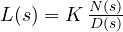 , with
 of degree
 (zeros
 ) and
 of degree
 (poles
 ). The closed-loop poles are the roots of

The root locus is the set of these roots as  goes from 0 to
 .
The magnitude and angle conditions. A point  belongs to the locus if and only if
 , that is

The angle condition decides where the locus lies, the magnitude condition which gain corresponds to each point.
Sketching rules
- The locus has
 branches, symmetric about the real axis.
- The branches start at the poles of
 (
 ) and end at the zeros (
 );
 branches go to infinity.
- On the real axis, the points belonging to the locus are those with an odd number of real poles and zeros to their right (from the angle condition: each pole or zero to the right contributes 180°, those to the left 0°, complex pairs cancel).
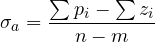
- Branches going to infinity follow asymptotes with angles
 , starting from the centroid
- Two branches meeting on the real axis break away at the points where
 (breakaway points).
- Crossings of the imaginary axis are found with the Routh criterion.
A complete example
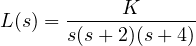
Three poles (0, −2, −4), no zeros.
- Real axis: the segment between 0 and −2 (one pole to the right) and everything to the left of −4 (three poles) belong to the locus.
- Asymptotes:
 , angles 60°, 180°, 300°, centroid
 .
- Breakaway:
 ,
 gives
 (the other root, −3.15, is not on the locus). There
 .
- Imaginary axis: from the lesson on stability,
 and
 .
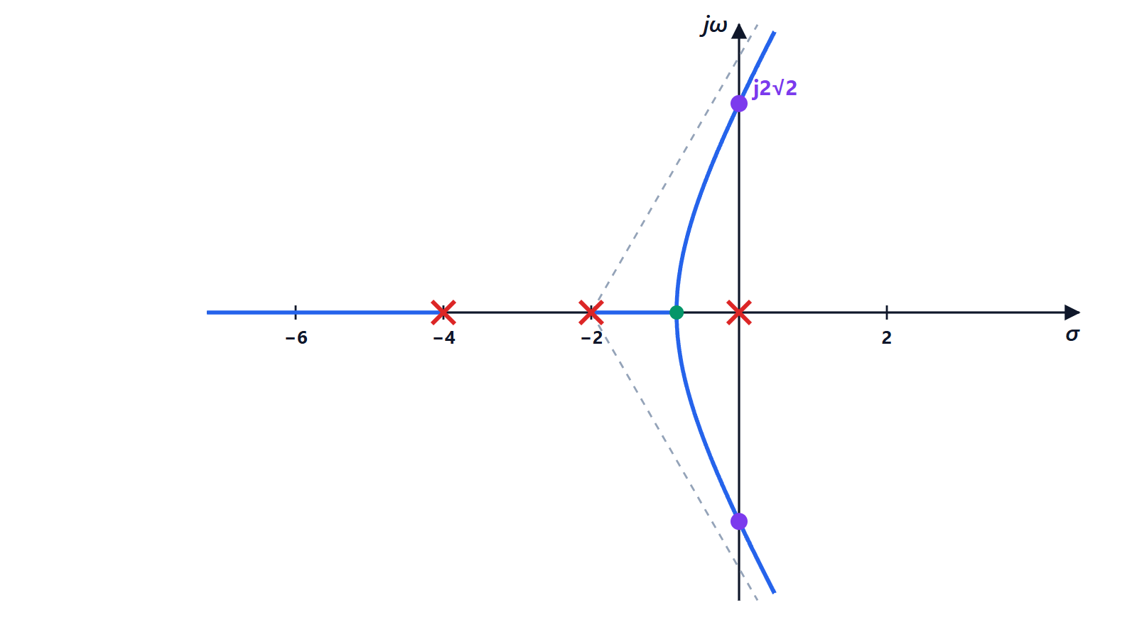
Reading the plot. For  the poles are real: a response without oscillation but slow. Between 3.08 and 48 the dominant pair is complex and less and less damped. For damping
 (16% overshoot) the poles must lie on the line at 60° from the negative real axis: the locus meets it at
 , with poles at
 ; the third pole is at
 , seven times further away, and the pair is truly dominant. The settling time is then about
 s, and it cannot be reduced by changing the gain alone: the real part of the complex poles never goes further left than −2, the centroid of the asymptotes.
Reshaping the locus
This is where the method is useful in design. Adding a zero to the controller attracts the branches and moves them to the left: with a zero at −2.5, for example, the asymptotes become two at ±90° with centroid  , and the loop stays stable for any gain. This is the effect of derivative action and of lead networks. Adding a pole (like the integrator) pushes the branches to the right and reduces stability. The root locus makes this trade-off visible, which is why, even in the age of simulation software, it remains the tool for reasoning about design.