Steady-state error, system type and integral action
The final value theorem, system type and error constants, the error table, integral action, disturbances and the internal model principle, the sensitivity trade-off.
A stable system, once the transient is over, reaches a steady state. But does the output follow the reference exactly, or is an error left? And how far do constant disturbances move the output? In this lesson we see how steady-state error is computed, the role of the system type, the error constants and why integral action removes the error for constant references.
The error and the final value theorem
From the feedback lesson, the error is

For the steady-state error  the final value theorem is used: if the limit exists (that is if the closed-loop system is stable),

System type
Write the loop function bringing out the poles at the origin (the integrators):
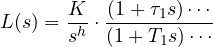
where the fraction on the right equals 1 at  . The number
 of integrators is the system type, and
 is the static (or generalised) gain.
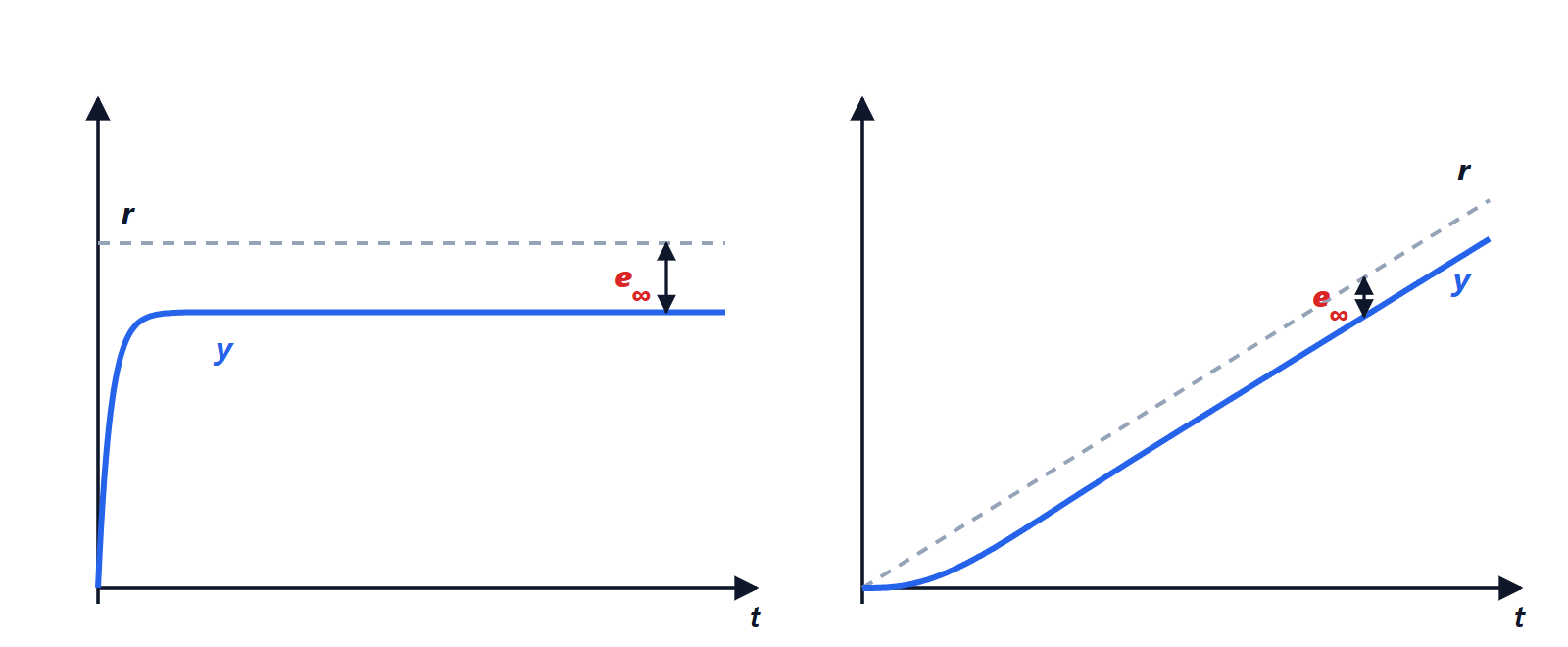
Step ( ):
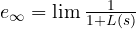 .
- type 0:
 , so
 ;
- type 1 or higher:
 , so
 .
Ramp ( ):
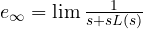 .
- type 0: infinite error, the output falls further and further behind;
- type 1:
 , so
 ;
- type 2 or higher: zero.
In summary:
| Type | Step | Ramp | Parabola |
|---|---|---|---|
| 0 |  |  | |
| 1 | 0 |  | |
| 2 | 0 | 0 | |
Example. A type 0 plant with loop gain  leaves an error of
 on a step. Getting down to 1% would need
 : but such a high gain often makes the loop unstable or too oscillatory (lesson on stability).
Integral action
The solution is to add an integrator in the controller:  , or better a PI,
 . The system becomes type 1 and the steady-state step error is zero, whatever the gain.
The intuitive reason: as long as there is even a small error, the integral keeps growing and the command with it; the system can come to rest only when the error is exactly zero. This is how a modern thermostat brings a room exactly to the set temperature, and cruise control holds the speed even uphill.
The price is one more pole at the origin, which adds 90° of phase lag to the loop function and tends to reduce stability: the controller must be designed with this in mind.
Disturbances
A constant disturbance  at the output produces in steady state, by the same formula, a shift of
 for a type 0 loop, zero if the loop is type 1. Where the disturbance enters matters: to remove in steady state a constant disturbance acting at the plant input (for example a load torque on a motor), the integrator must be in the controller, before the point where the disturbance enters. This is a case of the internal model principle: to track or reject a signal in steady state, the loop must contain a model of that signal (an integrator for constant signals, a pair of imaginary poles for sinusoids).
The fundamental trade-off
Since  , both cannot be made small at the same frequency. At low frequencies one wants
 small (good tracking and rejection of disturbances, which are slow); at high frequencies one wants
 small, so that sensor noise does not reach the output and because the plant model is unreliable there. The loop gain must therefore be high at low frequency and low at high frequency, with the transition between the two shaped so as not to compromise stability. This is the starting point of frequency-domain design, in the next lessons.