State space: state feedback and observers
State equations and the link with the transfer function, state feedback and pole placement on the inverted pendulum, controllability, LQR, observers and the Kalman filter.
Transfer functions describe the link between one input and one output. Many systems, however, have several inputs and outputs, and their internal state matters: a drone has four motors and six degrees of freedom, an inverted pendulum on a cart must be controlled by looking at position, angle and velocity together. The state-space representation describes the system with a set of first-order equations and makes it possible to design controllers that use all the internal quantities. In this lesson we cover state equations, controllability, state feedback with pole placement and observers.
State equations
The state  is the minimal set of quantities that, together with future inputs, determines the whole future evolution: positions and velocities of a mechanical system, capacitor voltages and inductor currents of a circuit. For a linear system:

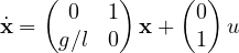
Example. An  -th order differential equation is brought into this form by choosing the output and its derivatives as states. For the inverted pendulum linearised around the upright position,
 (with
 the normalised command acceleration), with
 and
 :
The link with the transfer function. Taking the Laplace transform (zero initial conditions),  , so

The poles of  are the eigenvalues of
 , roots of
 . For the pendulum:
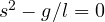 , eigenvalues
 , one positive: the inverted pendulum is unstable, as expected.
State feedback
If the whole state is measurable, the command  is used, with
 a row of gains. The closed loop becomes

and its poles are the eigenvalues of  , which can be chosen through .
Example. For the pendulum with  s⁻² and
 :

To have poles with  rad/s and
 , the desired polynomial is
 : so
 and
 . The command
 keeps the pendulum upright, with feedback on both angle and angular velocity: it is a PD controller, derived systematically.
Controllability. The poles can be placed at will if and only if the system is controllable, that is if the matrix

has rank . It means the input can influence every component of the state. For the pendulum 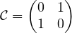 , of rank 2.
The inverted pendulum on a cart
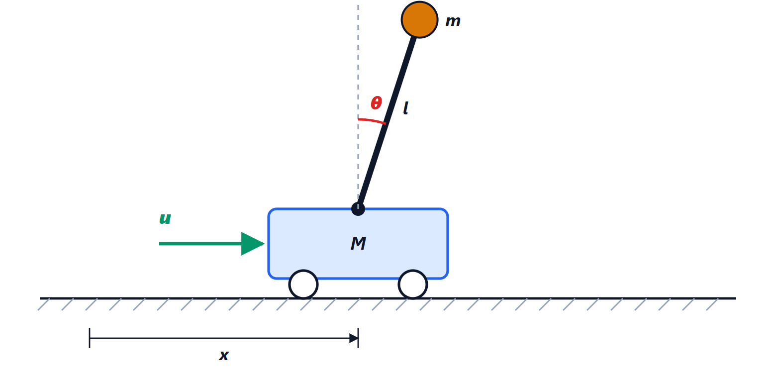
The classic case in control laboratories, and the principle of self-balancing vehicles like the Segway: a single input (the force on the cart) must control four states (cart position and velocity, rod angle and angular velocity). The linearised model is controllable, and state feedback with four gains manages to keep the rod upright and bring the cart back to the desired position. A single PID on the angle would not be enough: it would keep the rod straight, but the cart would drift away.
To choose the poles in a principled way the linear quadratic regulator (LQR) is often used, which computes the minimising a cost of the form  : an explicit trade-off between accuracy and control effort.
Observers
Often not all of the state is measurable: the angle is measured by a sensor, but not the angular velocity. An observer is then built, a model of the system running in parallel on the computer and corrected by the difference between the measured and the predicted output:

The estimation error  satisfies
 : by choosing
 the estimate can be made as fast as desired, provided the system is observable (the dual condition of controllability). By the separation principle the feedback and the observer can be designed independently, and the feedback applied to the estimated state. The Kalman filter, used in the navigation of aircraft, phones and drones to fuse data from accelerometers, gyroscopes and GPS, is an observer designed taking sensor noise into account.