The PID controller: tuning and implementation
Proportional, integral and derivative actions, comparison of responses, Ziegler-Nichols tuning with an example, derivative filter, anti-windup and microcontroller code.
The PID controller (proportional, integral, derivative) is by far the most used in industry: it regulates temperatures, pressures, flows, motor speeds, robot arm positions, drone altitude. It has only three parameters, can be tuned even without an accurate plant model and works well in most cases. In this lesson we see what the three actions mean, tuning methods and the practical details that make a real PID work.
The three actions

It is often written with time constants,  .
- Proportional: reacts to the current error. The larger
 , the quicker the response and the smaller the steady-state error, but the less damped the loop. On its own it leaves a steady-state error on type 0 plants.
- Integral: reacts to the error accumulated in the past. It removes the steady-state error for constant references and disturbances (lesson on errors), but adds phase lag and tends to cause oscillation.
- Derivative: reacts to how fast the error is changing, that is it “anticipates” where it is going. It adds phase lead and damping, but amplifies high-frequency noise.
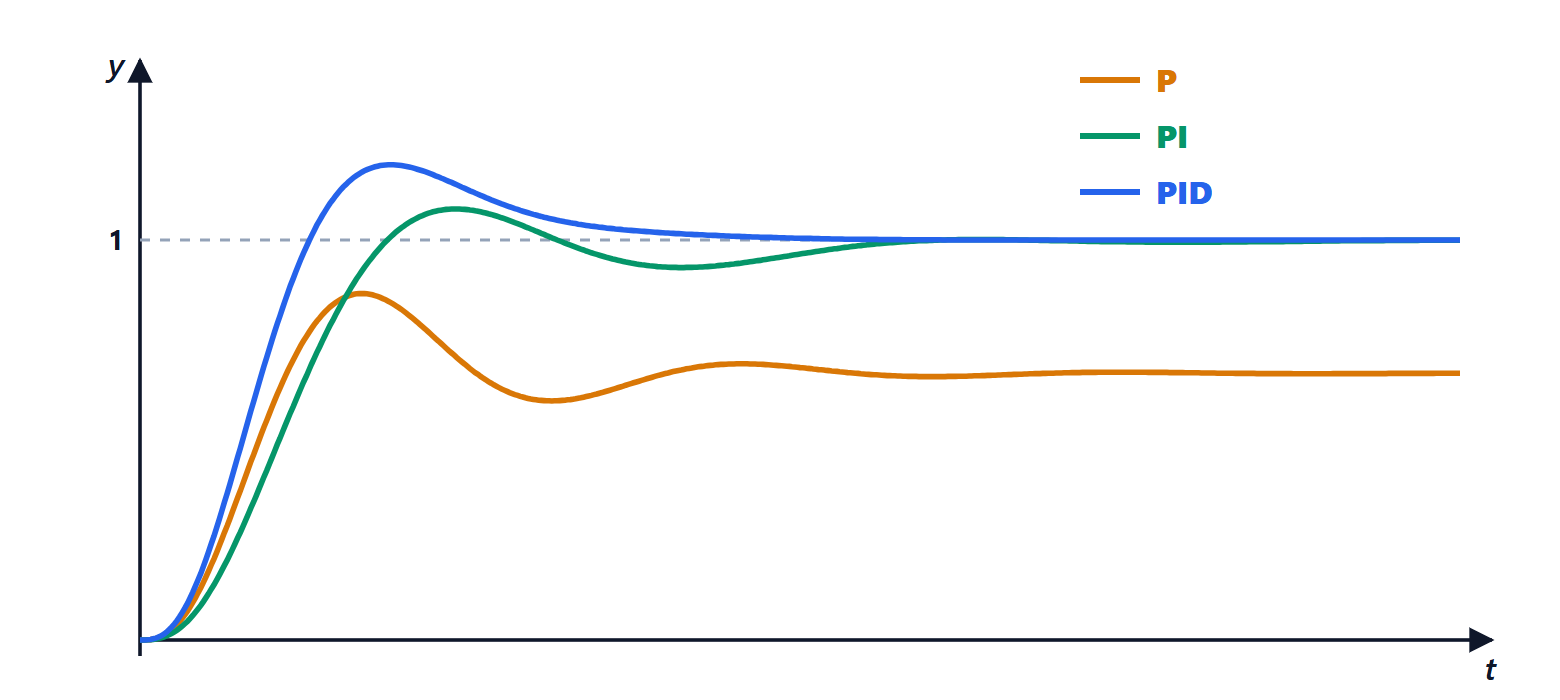
The figure shows typical behaviour on a plant  . With P alone (
 ) the output stops at
 : the steady-state error is
 . With PI it reaches 1 but more slowly. With PID it reaches 1, faster and with limited oscillation.
Ziegler-Nichols tuning
The classic method, from 1942, is applied directly to the plant:
- remove integral and derivative action and increase until the loop oscillates steadily;
- note the ultimate gain
 and the period of the oscillation
 ;
- choose the parameters from the table.
| Controller | |  |  |
|---|---|---|---|
| P |  | ||
| PI |  |  | |
| PID |  |  |  |
Example. For the ultimate gain is found with Routh: the characteristic equation is  , stable for
 , that is
 . At the limit the auxiliary equation
 gives
 , so
 s. The Ziegler-Nichols PID is
 ,
 s,
 s.
The Ziegler-Nichols rules give a quick but rather oscillatory response (overshoot often 30 to 50%): they are a good starting point to refine. Bringing a real plant to the edge of stability can be dangerous; there are variants using the open-loop step response, and modern industrial controllers have an autotuning function that runs a controlled test and computes the parameters by itself.
The details that matter
A PID written as in the formula works poorly in reality. The standard fixes are:
- Derivative filter. A pure derivative amplifies sensor noise. One uses
 , with
 about a tenth of , which limits the gain at high frequencies.
- Derivative on measurement. When the reference changes as a step, the derivative of the error is an impulse that gives the actuator a violent kick (the “derivative kick”). So only the measured output is differentiated,
 : for disturbances the effect is the same.
- Anti-windup. Every actuator has limits: a valve does not open beyond 100%, a motor has a maximum voltage. If the actuator is saturated the error does not shrink, but the integral keeps growing (windup); when the error finally changes sign, the huge integral takes a long time to unwind and the output overshoots the reference by a lot. The solution is to stop integrating while the command is saturated.
The PID in a microcontroller
In practice the PID is a program run at regular intervals  , much shorter than the plant time constants. The integral becomes a sum and the derivative a difference:
/* discrete-time PID with filtered derivative on measurement and anti-windup */
float kp = 4.8f, ki = 4.8f / 1.81f, kd = 4.8f * 0.45f;
float Ts = 0.01f, a = 0.1f;        /* sampling step and filter */
float integ = 0, d = 0, y_prev = 0;

float pid(float r, float y) {
    float e = r - y;
    d = (1 - a) * d - a * kd * (y - y_prev) / Ts;
    y_prev = y;
    float u = kp * e + integ + d;
    if (u > 10.0f) u = 10.0f;            /* actuator saturation */
    else if (u < -10.0f) u = -10.0f;
    else integ += ki * e * Ts;           /* integrate only when not saturated */
    return u;
}
That is all: a few multiplications per cycle. This is why a PID runs on any microcontroller, even the smallest, and is found inside household appliances, drones, 3D printers and digital power supplies.