Math Analysis 1

Solved limit exercises, from basic to exam level

Twenty-two exercises with solutions: standard limits, indeterminate forms, 1 to the infinity, squeezing, Taylor expansions, parameters, sequences and asymptotes, with graphs.

ielettronica 25 October 2026 12 min read 0 comments

Exercises on limits of functions and sequences of the kind set in Calculus 1 (Mathematical Analysis 1) courses, in three levels: basic, for the direct use of standard limits and elementary techniques; intermediate, with $1^\infty$ and $0\cdot\infty$ forms, changes of variable and squeezing; exam, with Taylor expansions, parameters and asymptotes, as in written exams and mid-term tests. The result is given straight away; the full solution opens with a click. The tables of standard limits and expansions are in the in-depth study linked at the top.

Basic level

Exercise 1. A standard limit with sine

Compute $\displaystyle\lim_{x\to 0}\frac{\sin 5x}{3x}$ .

Result: $\frac{5}{3}$ .

Solution

As $x \to 0$ also $5x \to 0$ , so $\sin 5x \sim 5x$ . Substituting in the quotient: $\dfrac{5x}{3x} = \dfrac{5}{3}$ .

Alternatively, without equivalences: 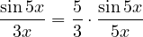$\dfrac{\sin 5x}{3x} = \dfrac{5}{3}\cdot\dfrac{\sin 5x}{5x}$ , and the second factor tends to 1.

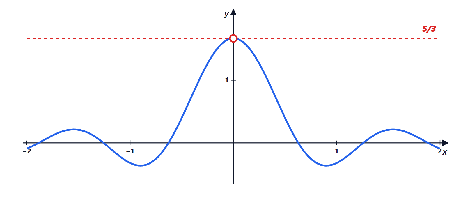
Graph for exercise 1 — The blue curve is sine of 5 x over 3 x; as x tends to 0 it approaches the dashed red line, the value of the limit: 5/3. The empty circle shows that the function is not defined at that point.

Exercise 2. Cosine and sine together

Compute $\displaystyle\lim_{x\to 0}\frac{1 - \cos x}{x\sin x}$ .

Result: $\frac{1}{2}$ .

Solution

Numerator and denominator are products and quotients of infinitesimals: they can be replaced by equivalents. $1 - \cos x \sim \frac{x^2}{2}$ and $x\sin x \sim x\cdot x = x^2$ . The limit is $\dfrac{x^2/2}{x^2} = \dfrac{1}{2}$ .

Graph for exercise 2 — The blue curve is 1 minus cosine of x over x times sine of x; as x tends to 0 it approaches the dashed red line, the value of the limit: 1/2. The empty circle shows that the function is not defined at that point.

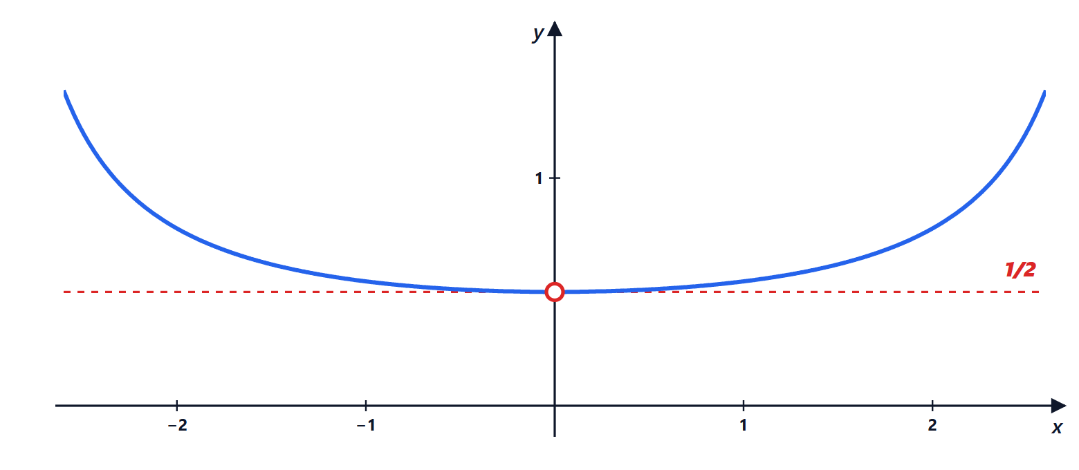
Exercise 3. Ratio of polynomials at infinity

Compute $\displaystyle\lim_{x\to+\infty}\frac{3x^2 - x + 1}{2x^2 + 5}$ .

Result: $\frac{3}{2}$ .

Solution

Form $\infty/\infty$ . Factor out the highest power above and below:

$\frac{x^2\left(3 - \frac{1}{x} + \frac{1}{x^2}\right)}{x^2\left(2 + \frac{5}{x^2}\right)} \to \frac{3}{2}$

General rule for ratios of polynomials at infinity: only the ratio of the highest-degree terms matters. With equal degrees you get the ratio of the coefficients; with a higher-degree numerator $\pm\infty$ ; with a higher-degree denominator 0.

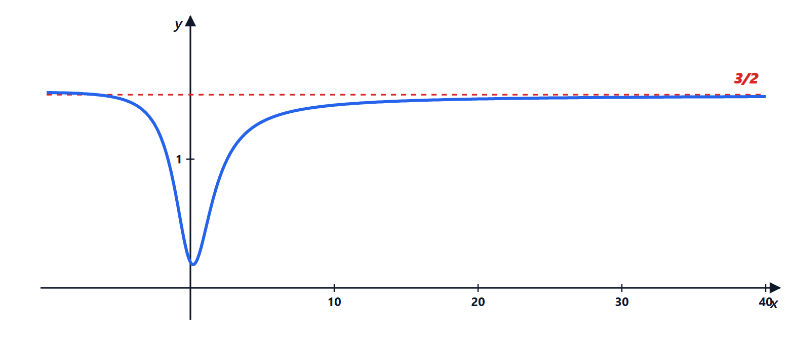
Graph for exercise 3 — The blue curve is the ratio of the two polynomials; as x tends to plus infinity it approaches the dashed red line, the value of the limit: 3/2.

Exercise 4. A difference of infinities with a square root

Compute $\displaystyle\lim_{x\to+\infty}\left(\sqrt{x^2 + x} - x\right)$ .

Result: $\frac{1}{2}$ .

Solution

Form $\infty - \infty$ . Rationalise by multiplying and dividing by $\sqrt{x^2 + x} + x$ :

$\sqrt{x^2 + x} - x = \frac{(x^2 + x) - x^2}{\sqrt{x^2 + x} + x} = \frac{x}{x\left(\sqrt{1 + \frac{1}{x}} + 1\right)} = \frac{1}{\sqrt{1 + \frac{1}{x}} + 1} \to \frac{1}{2}$

(For $x \gt 0$ , $\sqrt{x^2} = x$ ; as $x \to -\infty$ it would be $\sqrt{x^2} = -x$ and the limit would change: it becomes $+\infty$ .)

Graph for exercise 4 — The blue curve is square root of x squared plus x, minus x; as x tends to plus infinity it approaches the dashed red line, the value of the limit: 1/2.

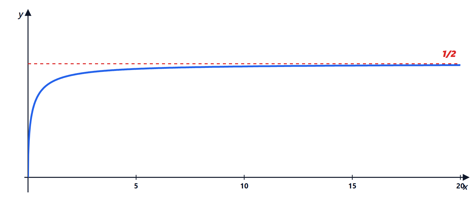
Exercise 5. Exponential and logarithm

Compute 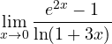$\displaystyle\lim_{x\to 0}\frac{e^{2x} - 1}{\ln(1 + 3x)}$ .

Result: $\frac{2}{3}$ .

Solution

$e^{2x} - 1 \sim 2x$ and $\ln(1 + 3x) \sim 3x$ . The limit is $\dfrac{2x}{3x} = \dfrac{2}{3}$ .

Graph for exercise 5 — The blue curve is e to the 2 x minus 1, over log of 1 plus 3 x; as x tends to 0 it approaches the dashed red line, the value of the limit: 2/3. The empty circle shows that the function is not defined at that point.

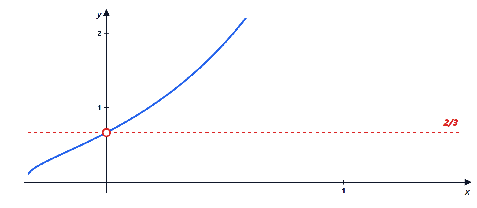
Exercise 6. Factor and simplify

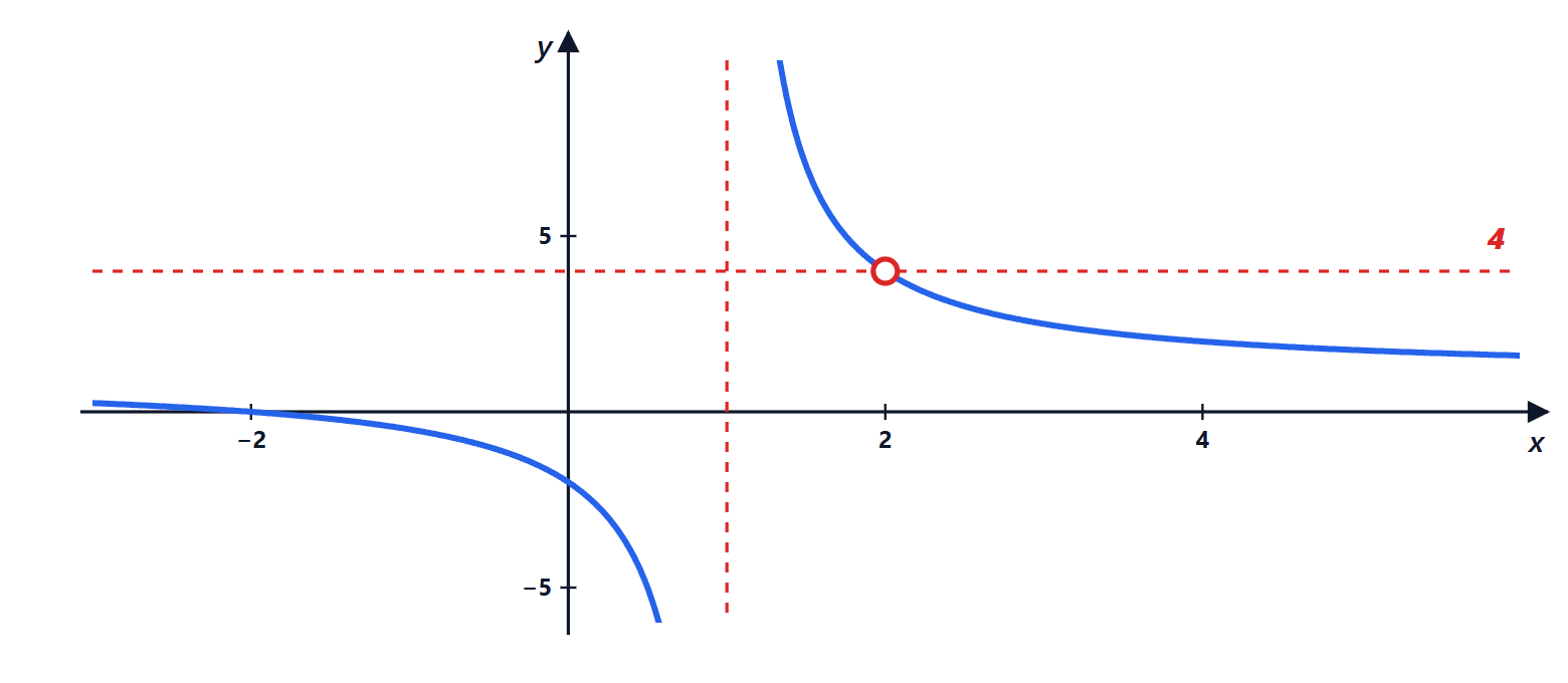
Compute 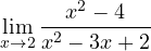$\displaystyle\lim_{x\to 2}\frac{x^2 - 4}{x^2 - 3x + 2}$ .

Result: 4.

Solution

Substituting $x = 2$ gives $0/0$ : both polynomials vanish at 2, so both are divisible by $x - 2$ (factor theorem).

$\frac{x^2 - 4}{x^2 - 3x + 2} = \frac{(x - 2)(x + 2)}{(x - 2)(x - 1)} = \frac{x + 2}{x - 1} \to \frac{4}{1} = 4$

Graph for exercise 6 — The blue curve is the ratio of the two polynomials, which has a vertical asymptote at x equal to 1; as x tends to 2 it approaches the dashed red line, the value of the limit: 4. The empty circle shows that the function is not defined at that point.

Intermediate level

Exercise 7. A 1 to the infinity form

Compute 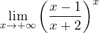$\displaystyle\lim_{x\to+\infty}\left(\frac{x - 1}{x + 2}\right)^x$ .

Result: $e^{-3}$ .

Solution

The base tends to 1 and the exponent to $+\infty$ : form $1^\infty$ . Write the base as 1 plus an infinitesimal: $\dfrac{x - 1}{x + 2} = 1 - \dfrac{3}{x + 2}$ .

Switch to the exponential: 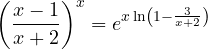$\left(\dfrac{x - 1}{x + 2}\right)^x = e^{x\ln\left(1 - \frac{3}{x + 2}\right)}$ . Since $\ln(1 + u) \sim u$ as $u \to 0$ :

$x\ln\left(1 - \frac{3}{x + 2}\right) \sim x\cdot\left(-\frac{3}{x + 2}\right) \to -3$

and the limit is $e^{-3}$ . The same result follows from the corollary $\left(1 + \frac{b}{x}\right)^x \to e^b$ , after noting that $x + 2 \sim x$ .

Graph for exercise 7 — The blue curve is x minus 1 over x plus 2, to the power x; as x tends to plus infinity it approaches the dashed red line, the value of the limit: e to the minus 3, about 0.05.

Exercise 8. When equivalences are not enough

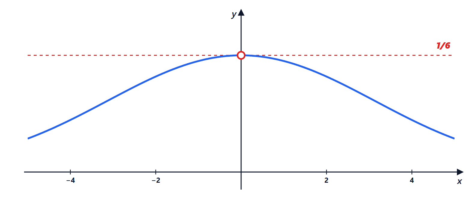
Compute $\displaystyle\lim_{x\to 0}\frac{x - \sin x}{x^3}$ .

Result: $\frac{1}{6}$ .

Solution

Substituting $\sin x \sim x$ in the numerator would give $x - x = 0$ : wrong, because in a difference the leading terms cancel. The next term of the expansion is needed: $\sin x = x - \frac{x^3}{6} + o(x^4)$ .

$\frac{x - \sin x}{x^3} = \frac{\frac{x^3}{6} + o(x^4)}{x^3} = \frac{1}{6} + o(x) \to \frac{1}{6}$

With l’Hôpital’s rule (allowed: form 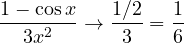$0/0$ ): $\dfrac{1 - \cos x}{3x^2} \to \dfrac{1/2}{3} = \dfrac{1}{6}$ .

Graph for exercise 8 — The blue curve is x minus sine of x, over x cubed; as x tends to 0 it approaches the dashed red line, the value of the limit: 1/6. The empty circle shows that the function is not defined at that point.

Exercise 9. The logarithm of cosine

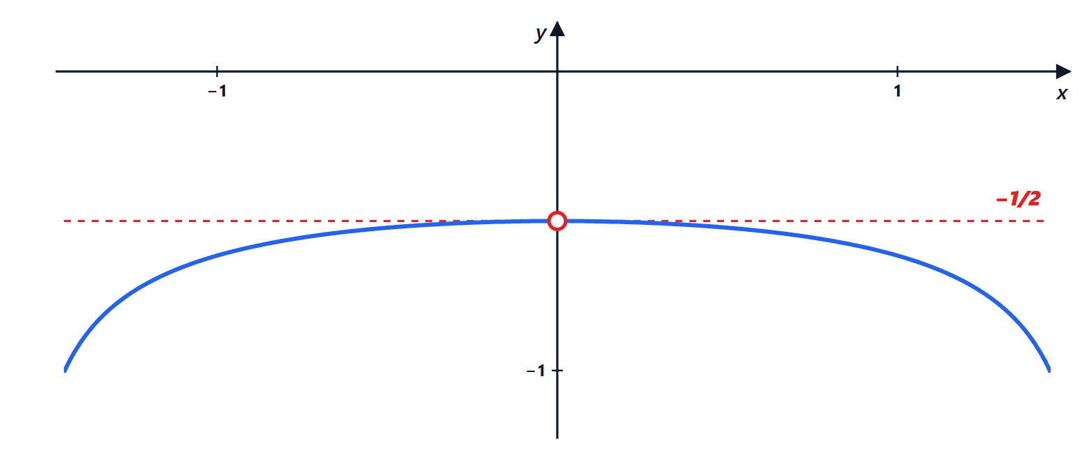
Compute $\displaystyle\lim_{x\to 0}\frac{\ln(\cos x)}{x^2}$ .

Result: $-\frac{1}{2}$ .

Solution

Write $\cos x = 1 + (\cos x - 1)$ , with $u = \cos x - 1 \to 0$ . Then $\ln(\cos x) = \ln(1 + u) \sim u = \cos x - 1 \sim -\dfrac{x^2}{2}$ .

The limit is 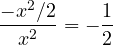$\dfrac{-x^2/2}{x^2} = -\dfrac{1}{2}$ . This step comes up often: $\ln f \sim f - 1$ when $f \to 1$ .

Graph for exercise 9 — The blue curve is log of cosine of x over x squared; as x tends to 0 it approaches the dashed red line, the value of the limit: minus 1/2. The empty circle shows that the function is not defined at that point.

Exercise 10. Zero times infinity

Compute $\displaystyle\lim_{x\to 0^+}x\ln x$ .

Result: 0.

Solution

Form $0\cdot(-\infty)$ . Set $x = 1/t$ , with $t \to +\infty$ : $x\ln x = \dfrac{1}{t}\ln\dfrac{1}{t} = -\dfrac{\ln t}{t} \to 0$ , by the hierarchy of infinities (the logarithm is negligible compared with any power).

More generally $x^\alpha\ln x \to 0$ as $x \to 0^+$ for every $\alpha \gt 0$ : the power “wins” near zero too.

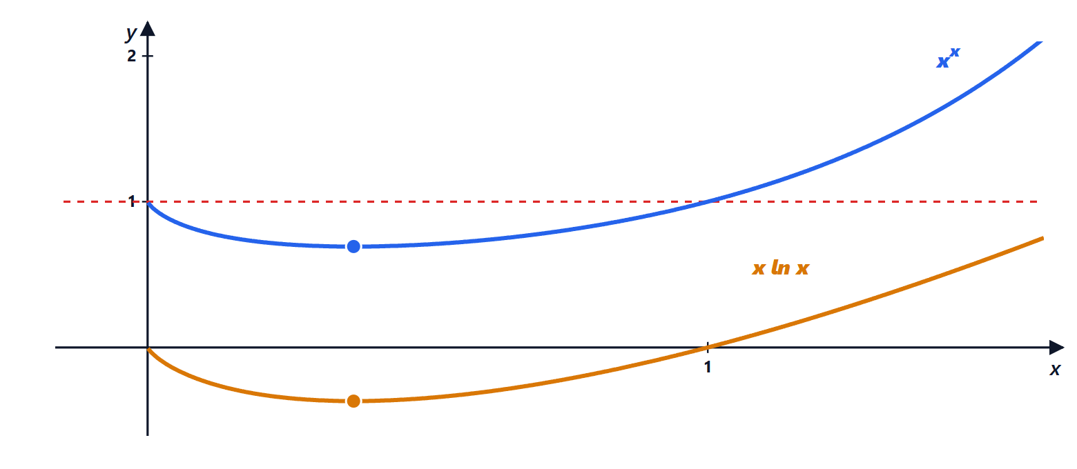
Graphs of x times log x and of x to the x — The orange curve, x log x, tends to zero as x tends to zero from the right and has a minimum of minus 1 over e at x equal to 1 over e. The blue curve, x to the x, which is e raised to the orange curve, tends to 1 and has its minimum at x equal to 1 over e.

Exercise 11. Zero to the zero

Compute $\displaystyle\lim_{x\to 0^+}x^x$ .

Result: 1.

Solution

Form $0^0$ . Switch to the exponential: $x^x = e^{x\ln x}$ . The exponent tends to 0 (previous exercise) and the exponential is continuous, so $x^x \to e^0 = 1$ .

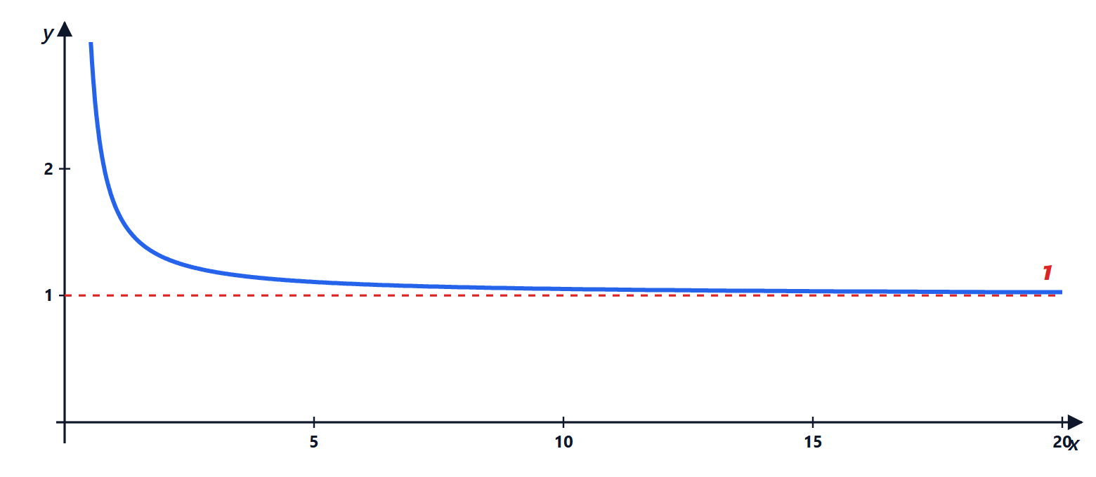
Exercise 12. A change of variable at infinity

Compute $\displaystyle\lim_{x\to+\infty}x\left(e^{1/x} - 1\right)$ .

Result: 1.

Solution

Form $\infty\cdot 0$ . With $t = 1/x \to 0^+$ : $x\left(e^{1/x} - 1\right) = \dfrac{e^t - 1}{t} \to 1$ .

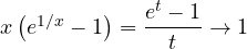This is an example of the rule: when $x \to \infty$ , the change $t = 1/x$ brings the standard limits back “to 0”.

Graph for exercise 12 — The blue curve is x times e to the 1 over x minus 1; as x tends to plus infinity it approaches the dashed red line, the value of the limit: 1.

Exercise 13. Moving to the right point

Compute 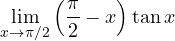$\displaystyle\lim_{x\to\pi/2}\left(\frac{\pi}{2} - x\right)\tan x$ .

Result: 1.

Solution

The standard limits are “at 0”: set $t = \frac{\pi}{2} - x \to 0$ . Then $\tan x = \tan\left(\frac{\pi}{2} - t\right) = \dfrac{\cos t}{\sin t}$ (complementary-angle formulas).

$\left(\frac{\pi}{2} - x\right)\tan x = t\cdot\frac{\cos t}{\sin t} = \frac{t}{\sin t}\cdot\cos t \to 1\cdot 1 = 1$

The limit is the same from the right and from the left: for $x \gt \pi/2$ both $t$ and $\tan x$ are negative.

Graph for exercise 13 — The blue curve is pi over 2 minus x, times tangent of x; as x tends to pi over 2 it approaches the dashed red line, the value of the limit: 1. The empty circle shows that the function is not defined at that point.

Exercise 14. A ratio of logarithms

Compute 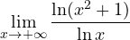$\displaystyle\lim_{x\to+\infty}\frac{\ln(x^2 + 1)}{\ln x}$ .

Result: 2.

Solution

Factor $x^2$ out inside the logarithm: $\ln(x^2 + 1) = \ln\left[x^2\left(1 + \frac{1}{x^2}\right)\right] = 2\ln x + \ln\left(1 + \frac{1}{x^2}\right)$ .

The second term tends to 0, so $\dfrac{\ln(x^2 + 1)}{\ln x} = 2 + \dfrac{\ln(1 + 1/x^2)}{\ln x} \to 2$ .

Graph for exercise 14 — The blue curve is log of x squared plus 1 over log of x; as x tends to plus infinity it approaches the dashed red line, the value of the limit: 2.

Exercise 15. The squeeze theorem

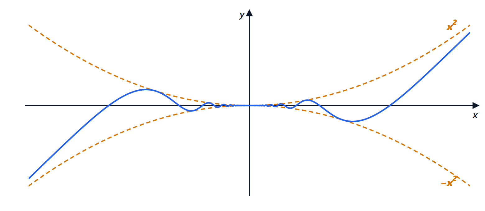
Compute 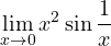$\displaystyle\lim_{x\to 0}x^2\sin\frac{1}{x}$ .

Result: 0.

Solution

$\sin(1/x)$ has no limit as $x \to 0$ : it oscillates between $-1$ and 1 faster and faster. But it is bounded: $\left|\sin\frac{1}{x}\right| \le 1$ , so

$-x^2 \le x^2\sin\frac{1}{x} \le x^2$

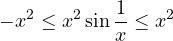
Both bounds tend to 0, and by the squeeze theorem so does the middle function. Useful rule: an infinitesimal times a bounded function is an infinitesimal.

The function x squared times sine of 1 over x squeezed between two parabolas — The blue curve oscillates faster and faster near the origin, but stays between the parabolas minus x squared and x squared, in orange, which both tend to zero and force it to do the same.

Exam level

Exercise 16. Taylor with a square root

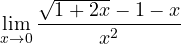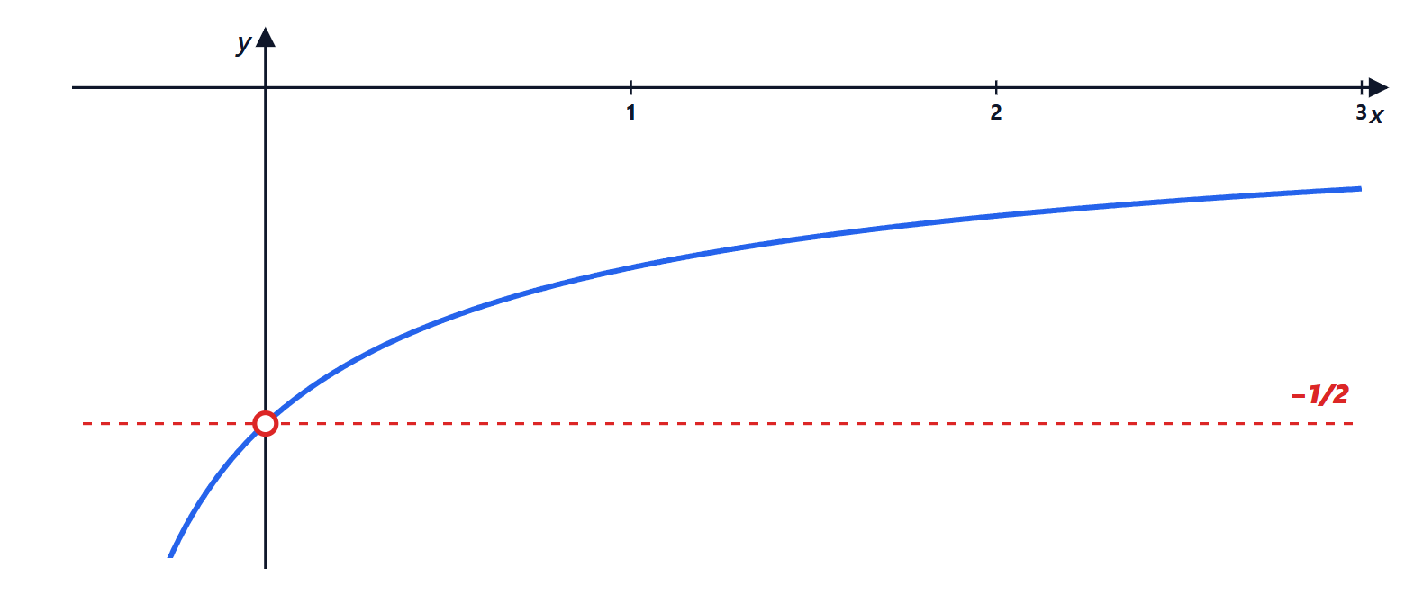
Compute $\displaystyle\lim_{x\to 0}\frac{\sqrt{1 + 2x} - 1 - x}{x^2}$ .

Result: $-\frac{1}{2}$ .

Solution

The equivalence $\sqrt{1 + 2x} - 1 \sim x$ would cancel the $-x$ and give 0: a mistake. Expand to second order $(1 + u)^{1/2} = 1 + \frac{u}{2} - \frac{u^2}{8} + o(u^2)$ with $u = 2x$ :

$\sqrt{1 + 2x} = 1 + x - \frac{4x^2}{8} + o(x^2) = 1 + x - \frac{x^2}{2} + o(x^2)$

Numerator: 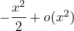$-\dfrac{x^2}{2} + o(x^2)$ . The limit is $-\dfrac{1}{2}$ .

Graph for exercise 16 — The blue curve is square root of 1 plus 2 x, minus 1 minus x, over x squared; as x tends to 0 it approaches the dashed red line, the value of the limit: minus 1/2. The empty circle shows that the function is not defined at that point.

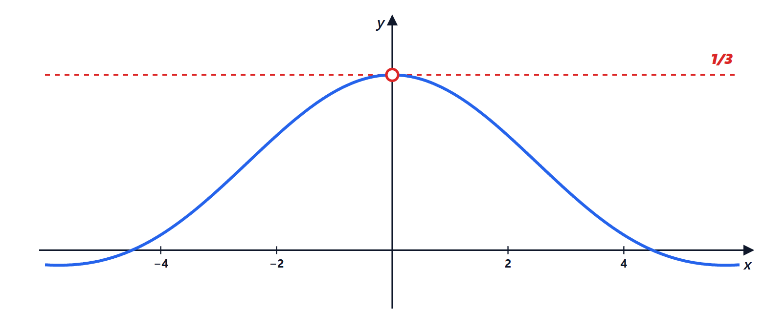
Exercise 17. Sine minus x times cosine

Compute $\displaystyle\lim_{x\to 0}\frac{\sin x - x\cos x}{x^3}$ .

Result: $\frac{1}{3}$ .

Solution

The denominator is of order 3, so expand the numerator up to order 3:

$\sin x = x - \frac{x^3}{6} + o(x^3)$ ; $x\cos x = x\left(1 - \frac{x^2}{2} + o(x^2)\right) = x - \frac{x^3}{2} + o(x^3)$ .

Difference: $-\frac{x^3}{6} + \frac{x^3}{2} + o(x^3) = \frac{x^3}{3} + o(x^3)$ . The limit is $\dfrac{1}{3}$ .

Practical rule: expand each term up to the order of the denominator (or up to the first order that does not cancel).

Graph for exercise 17 — The blue curve is sine of x minus x cosine of x, over x cubed; as x tends to 0 it approaches the dashed red line, the value of the limit: 1/3. The empty circle shows that the function is not defined at that point.

Exercise 18. Difference of two infinities with Taylor

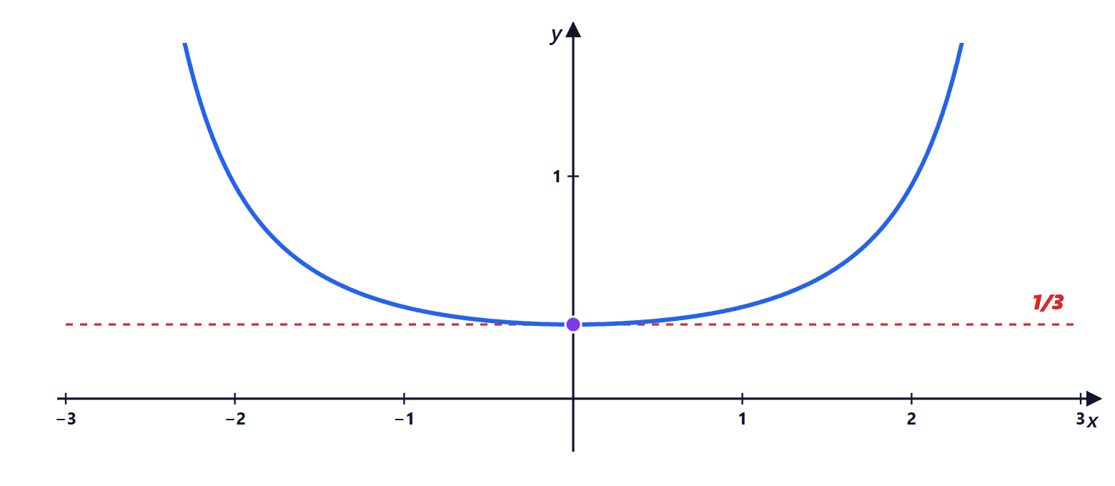
Compute 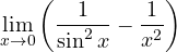$\displaystyle\lim_{x\to 0}\left(\frac{1}{\sin^2 x} - \frac{1}{x^2}\right)$ .

Result: $\frac{1}{3}$ .

Solution

Form $\infty - \infty$ . Common denominator:

$\frac{1}{\sin^2 x} - \frac{1}{x^2} = \frac{x^2 - \sin^2 x}{x^2\sin^2 x}$

The denominator is $\sim x^2\cdot x^2 = x^4$ . In the numerator: $\sin^2 x = \left(x - \frac{x^3}{6} + o(x^3)\right)^2 = x^2 - \frac{x^4}{3} + o(x^4)$ (the cross term is $2\cdot x\cdot\left(-\frac{x^3}{6}\right) = -\frac{x^4}{3}$ ).

Numerator: $\frac{x^4}{3} + o(x^4)$ . The limit is $\dfrac{x^4/3}{x^4} = \dfrac{1}{3}$ .

Graph of 1 over sine squared of x minus 1 over x squared — The two separate functions blow up at zero, but their difference stays bounded and tends to one third, shown by the dashed line.

Exercise 19. A 1 to the infinity form with cosine

Compute 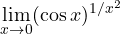$\displaystyle\lim_{x\to 0}(\cos x)^{1/x^2}$ .

Result: 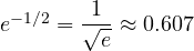$e^{-1/2} = \dfrac{1}{\sqrt e} \approx 0.607$ .

Solution

$(\cos x)^{1/x^2} = e^{\ln(\cos x)/x^2}$ . The exponent tends to $-\frac{1}{2}$ (exercise 9), so the limit is $e^{-1/2}$ .

Graph for exercise 19 — The blue curve is cosine of x to the power 1 over x squared; as x tends to 0 it approaches the dashed red line, the value of the limit: 1 over root e, about 0.607. The empty circle shows that the function is not defined at that point.

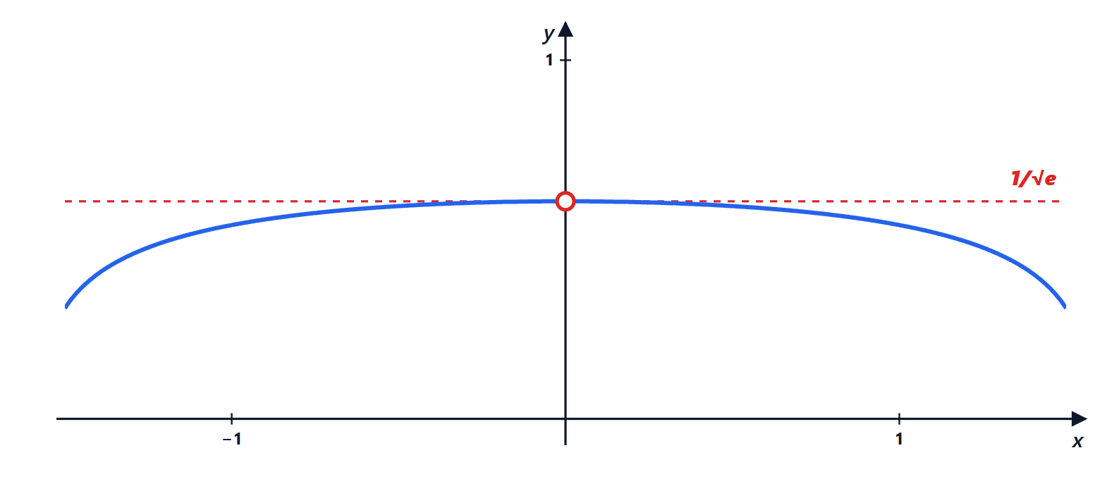
Exercise 20. Finding the parameters

Find the real numbers $a$ and $b$ for which the limit 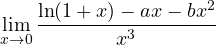$\displaystyle\lim_{x\to 0}\frac{\ln(1 + x) - ax - bx^2}{x^3}$ is finite, and compute it.

Result: $a = 1$ , $b = -\frac{1}{2}$ ; the limit is $\frac{1}{3}$ .

Solution

Expansion: $\ln(1 + x) = x - \frac{x^2}{2} + \frac{x^3}{3} + o(x^3)$ . The numerator is

$(1 - a)x + \left(-\frac{1}{2} - b\right)x^2 + \frac{x^3}{3} + o(x^3)$

Divided by $x^3$ : $\dfrac{1 - a}{x^2} + \dfrac{-\frac{1}{2} - b}{x} + \dfrac{1}{3} + o(1)$ .

1. If $a \ne 1$ , the first term dominates and the limit is infinite.

2. If $a = 1$ but $b \ne -\frac{1}{2}$ , the second term dominates: it tends to $+\infty$ on one side and to $-\infty$ on the other, so the limit does not exist.

3. With $a = 1$ and $b = -\frac{1}{2}$ what remains is $\frac{1}{3} + o(1)$ : the limit is $\frac{1}{3}$ .

Meaning: $x - \frac{x^2}{2}$ is the second-order Taylor polynomial of the logarithm, the only one that approximates $\ln(1 + x)$ with an error of order $x^3$ .

Graph for exercise 20 — The blue curve is the ratio with a equal to 1 and b equal to minus 1/2; as x tends to 0 it approaches the dashed red line, the value of the limit: 1/3. The empty circle shows that the function is not defined at that point.

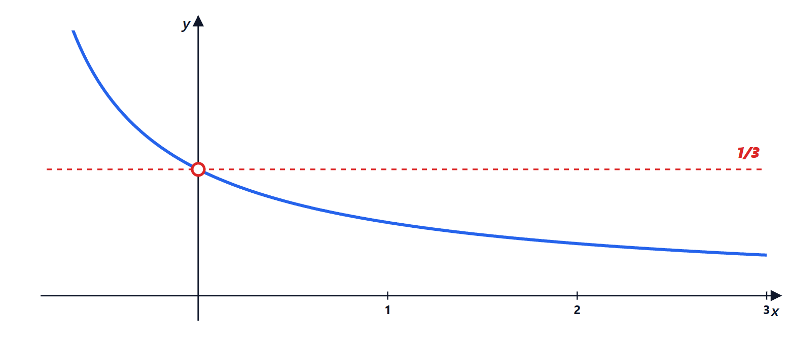
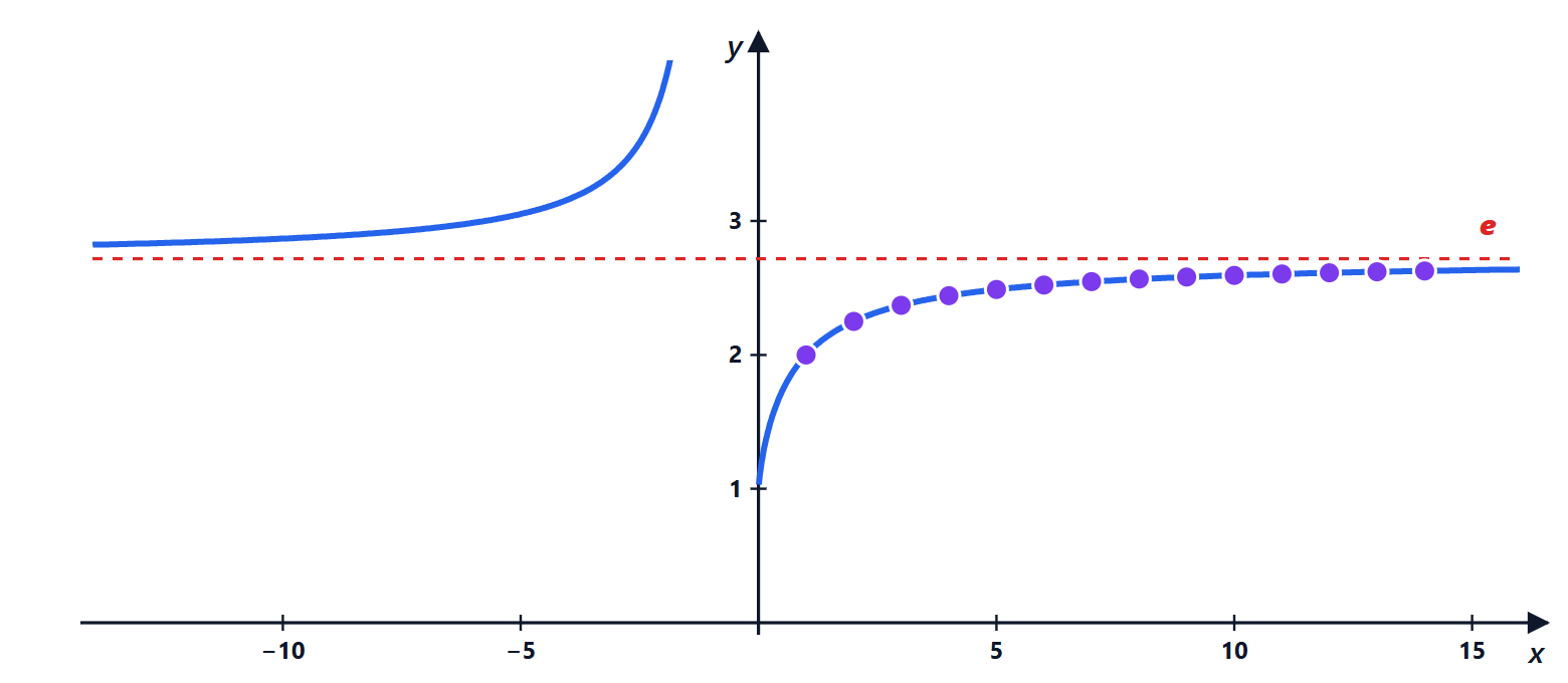
Exercise 21. The limit of a sequence

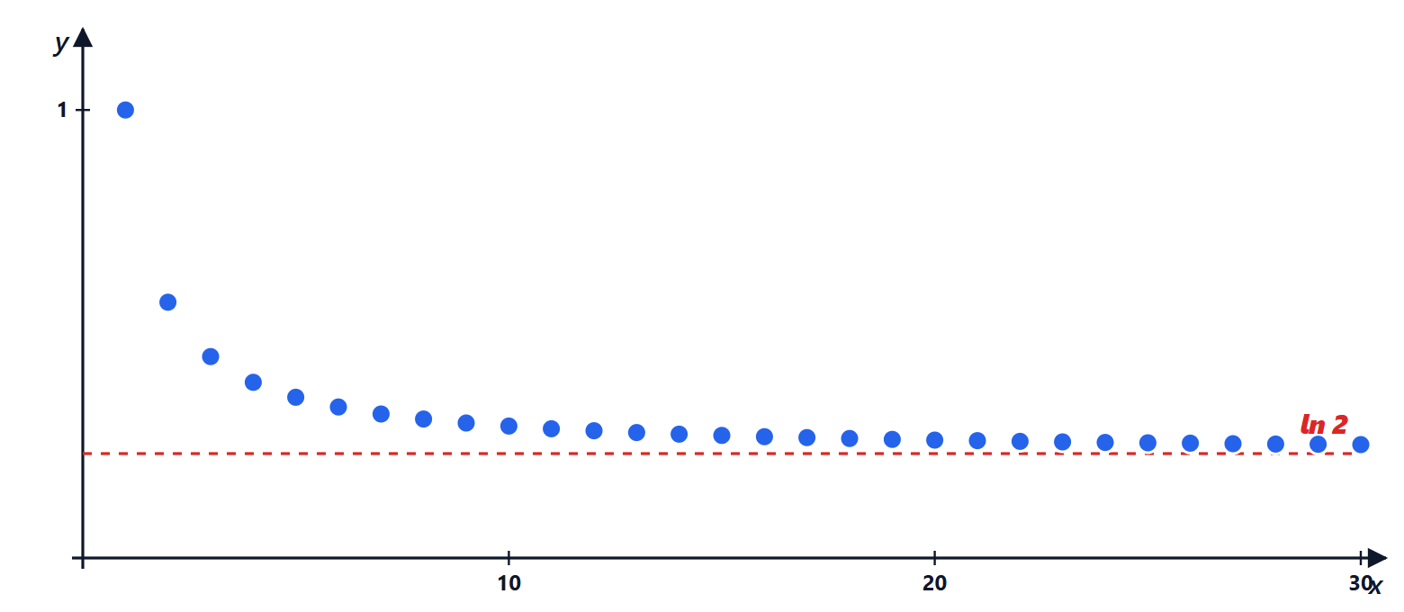
Compute 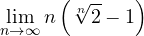$\displaystyle\lim_{n\to\infty}n\left(\sqrt[n]{2} - 1\right)$ .

Result: $\ln 2 \approx 0.693$ .

Solution

Form $\infty\cdot 0$ . Write $\sqrt[n]{2} = 2^{1/n}$ and set $t = 1/n \to 0^+$ :

$n\left(2^{1/n} - 1\right) = \frac{2^t - 1}{t} \to \ln 2$

Passing from the sequence to the function is allowed by the sequential characterisation of limits (lesson on sequences): if the limit of the function exists, the sequence has the same limit.

Graph for exercise 21 — The blue curve is the terms of the sequence n times the n-th root of 2 minus 1; as n grows it approaches the dashed red line, the value of the limit: log 2, about 0.693.

Exercise 22. Asymptotes of a rational function

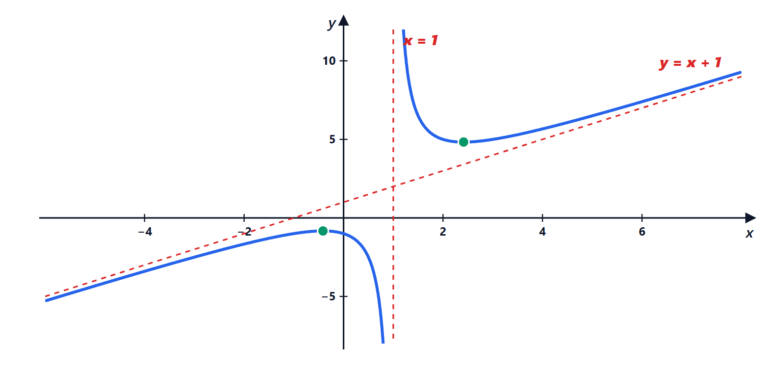
Find the asymptotes of 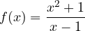$f(x) = \dfrac{x^2 + 1}{x - 1}$ and determine on which side of the graph the oblique asymptote lies.

Result: vertical asymptote $x = 1$ ; oblique asymptote $y = x + 1$ , with the graph above the asymptote for $x \gt 1$ and below it for $x \lt 1$ .

Solution

Vertical. The domain is $x \ne 1$ . As $x \to 1$ the numerator tends to 2 and the denominator to 0: $f \to +\infty$ as $x \to 1^+$ and $f \to -\infty$ as $x \to 1^-$ . So $x = 1$ is a vertical asymptote.

Horizontal. As $x \to \pm\infty$ , $f(x) \sim x \to \pm\infty$ : there is none.

Oblique. $m = \lim\dfrac{f(x)}{x} = \lim\dfrac{x^2 + 1}{x^2 - x} = 1$ ; $q = \lim\left(f(x) - x\right) = \lim\dfrac{x^2 + 1 - x^2 + x}{x - 1} = \lim\dfrac{x + 1}{x - 1} = 1$ . Asymptote $y = x + 1$ , both at $+\infty$ and at $-\infty$ .

Position. By polynomial division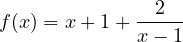: $x^2 + 1 = (x - 1)(x + 1) + 2$ , so $f(x) = x + 1 + \dfrac{2}{x - 1}$ . The difference 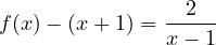$f(x) - (x + 1) = \dfrac{2}{x - 1}$ is positive for $x \gt 1$ (graph above the asymptote) and negative for $x \lt 1$ (below).

For rational functions whose numerator degree is the denominator degree plus one, division gives the oblique asymptote and the position straight away, without computing limits.

Graph of x squared plus 1 over x minus 1 with its asymptotes — The vertical asymptote x equal to 1 and the oblique asymptote y equal to x plus 1 are dashed. The right branch lies above the oblique asymptote and has a minimum, the left one lies below and has a maximum.

0 Comments

Oldest

Newest Most Voted

Cookie	Duration	Description
cookielawinfo-checkbox-analytics	11 months	This cookie is set by GDPR Cookie Consent plugin. The cookie is used to store the user consent for the cookies in the category "Analytics".
cookielawinfo-checkbox-functional	11 months	The cookie is set by GDPR cookie consent to record the user consent for the cookies in the category "Functional".
cookielawinfo-checkbox-necessary	11 months	This cookie is set by GDPR Cookie Consent plugin. The cookies is used to store the user consent for the cookies in the category "Necessary".
cookielawinfo-checkbox-others	11 months	This cookie is set by GDPR Cookie Consent plugin. The cookie is used to store the user consent for the cookies in the category "Other.
cookielawinfo-checkbox-performance	11 months	This cookie is set by GDPR Cookie Consent plugin. The cookie is used to store the user consent for the cookies in the category "Performance".
viewed_cookie_policy	11 months	The cookie is set by the GDPR Cookie Consent plugin and is used to store whether or not user has consented to the use of cookies. It does not store any personal data.

Basic level

Exercise 1. A standard limit with sine

Exercise 2. Cosine and sine together

Exercise 3. Ratio of polynomials at infinity

Exercise 4. A difference of infinities with a square root

Exercise 5. Exponential and logarithm

Exercise 6. Factor and simplify

Intermediate level

Exercise 7. A 1 to the infinity form

Exercise 8. When equivalences are not enough

Exercise 9. The logarithm of cosine

Exercise 10. Zero times infinity

Exercise 11. Zero to the zero

Exercise 12. A change of variable at infinity

Exercise 13. Moving to the right point

Exercise 14. A ratio of logarithms

Exercise 15. The squeeze theorem

Exam level

Exercise 16. Taylor with a square root

Exercise 17. Sine minus x times cosine

Exercise 18. Difference of two infinities with Taylor

Exercise 19. A 1 to the infinity form with cosine

Exercise 20. Finding the parameters

Exercise 21. The limit of a sequence

Exercise 22. Asymptotes of a rational function

Related articles

Solved integral exercises, from basic to exam level

Solved residue theorem exercises: real integrals computed in the complex plane

Limits in depth: the number e, the hierarchy of infinities, little-o and the tables to remember

From real to complex and back: real integrals with residues, Jordan's lemma and all the contours

Solved curve-sketching exercises, with graphs

Solved Laplace transform exercises: differential equations, circuits and systems