From real to complex and back: real integrals with residues, Jordan's lemma and all the contours
Semicircle for rational functions, Jordan's lemma proved, the integral of sine x over x with the indented contour, keyhole, sector and Fresnel integrals, rectangle and Gaussian, trigonometric integrals, sum of the series of reciprocal squares.
This page goes deeper into the lesson on the residue theorem with the most spectacular application of complex analysis: computing real integrals by going through the complex plane. An integral along a line, often impossible with the methods of Calculus 1, becomes part of an integral along a closed curve; the residue theorem computes it with a little algebra; an estimate makes the extra pieces vanish; and one returns to the real line with the result. All the classical techniques are covered, each with its own contour: the semicircle, Jordan’s lemma, the indented contour, the keyhole, the sector, the rectangle, and finally the summation of a series.
The strategy
- Choose a complex function
 that coincides with the integrand on the real axis (or has the integrand as its real or imaginary part).
- Choose a closed curve that contains the real stretch
 (or
 ) and “closes” it with other pieces.
- By the residue theorem,
 at the poles inside the curve.
- Show, with the ML estimate or Jordan’s lemma, that the added pieces tend to zero (or to something known) as
 .
- The limit of the real stretch is the integral sought.
Rational functions: the semicircle
Theorem. Let  ,
 be polynomials with
 and with no real roots. Then

Proof. Integrate on the contour formed by and the semicircle  in the upper half-plane. For
 large enough all the poles of the upper half-plane are inside. On , since the denominator has degree at least 2 more,
 for some constant
 ; the length is
 ; by the ML estimate
 . ∎
Example.  . The poles of
 are the fourth roots of
 :
 ,
 in the upper half-plane. At a simple pole
 of
 ,
 (because
 ). Sum:
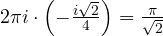
 . So the integral is
 .

Jordan’s lemma and Fourier integrals
For  one uses
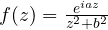 , with
 : on the real axis its real part is the integrand, and in the upper half-plane
 . When the denominator has degree only one more than the numerator the ML estimate is not enough, and a finer result is needed.
Jordan’s lemma. If  on with
 and , then
 .
Proof. With  :
 , so
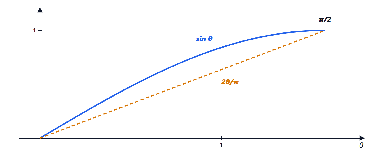
 . On
 we have
 (sine is concave and lies above the chord), so the integral is at most
 . In total
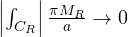 . ∎
Example. 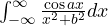 with
 . Only pole in the upper half-plane:
 , with residue
 . The integral of
 along the line is
 ; it is real, so it is exactly the integral of the cosine (that of the sine is zero, by symmetry). The result decays exponentially in
 : it is the Fourier transform of the Lorentzian (Fourier transform exercises).
The indented contour: the integral of 
Theorem. 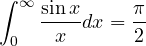 .
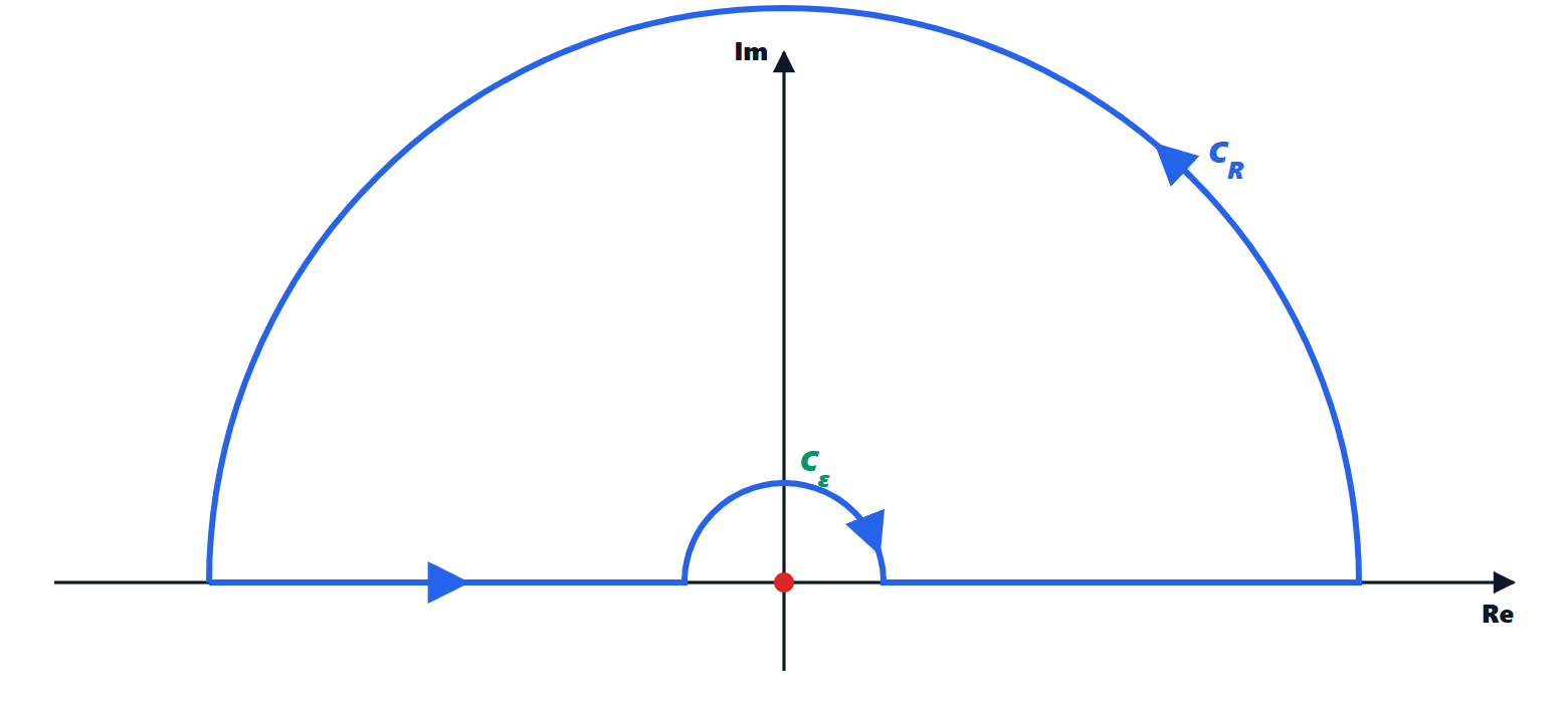
The sine integral has no elementary antiderivative. Use  , which has a pole on the real axis, at 0. The contour goes round it with a small semicircle
 above zero, traversed clockwise, and is closed with the large . There are no poles inside, so the total integral is zero.
Small semicircle lemma. If has a simple pole at  , the integral over a semicircle of radius
 around , traversed clockwise, tends to
 .
Proof. Near the pole  , with
 holomorphic and hence bounded: its integral over the arc tends to 0 by the ML estimate (the length is
 ). For the first term, with
 ,
 from
 to 0:
 . ∎
Proof of the theorem. On the contour:  . The piece on tends to 0 by Jordan (
 ,
 ); the one on tends to
 (residue of
 at 0). The two real stretches give, joining
 and
 ,
 . In the limit:
 , i.e.
 . ∎
The keyhole: non-integer powers
Theorem. For  :
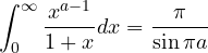 .
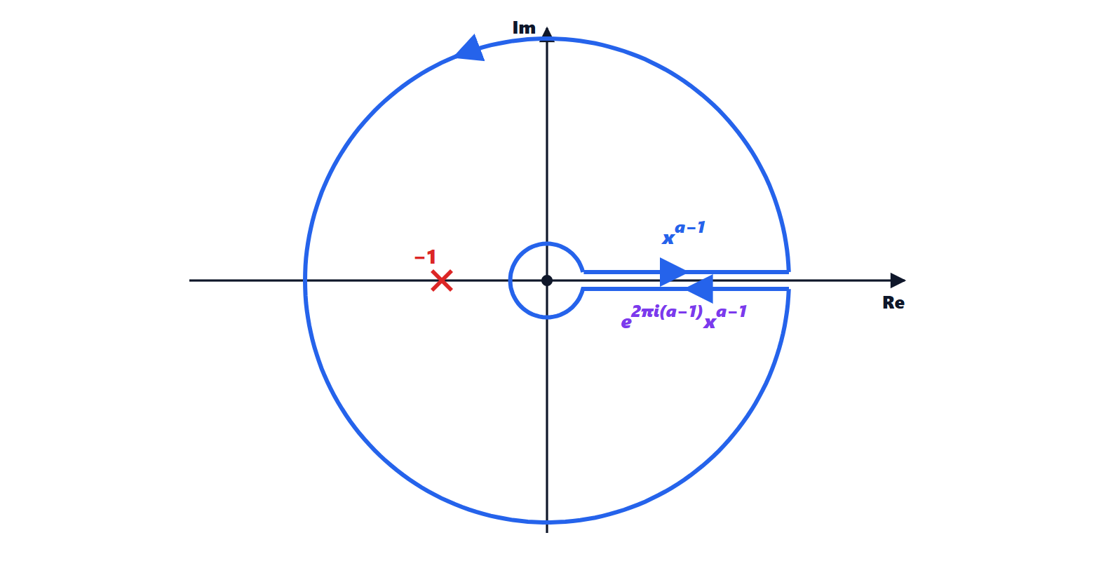
Proof. The function  is multivalued: choose the argument in
 , with the branch cut along the positive real half-axis. The “keyhole” contour runs along the upper edge of the cut from to , the large circle, the lower edge from to and the small circle. On the upper edge
 ; on the lower one the argument is
 , so
 .
The circles do not contribute in the limit: on the small one the integrand is about  and the length
 , product
 ; on the large one
 . Only pole:
 , with residue
 . So

∎ With  :
 . It is also the reflection formula of the Gamma function,
 .
The sector: exploiting a symmetry
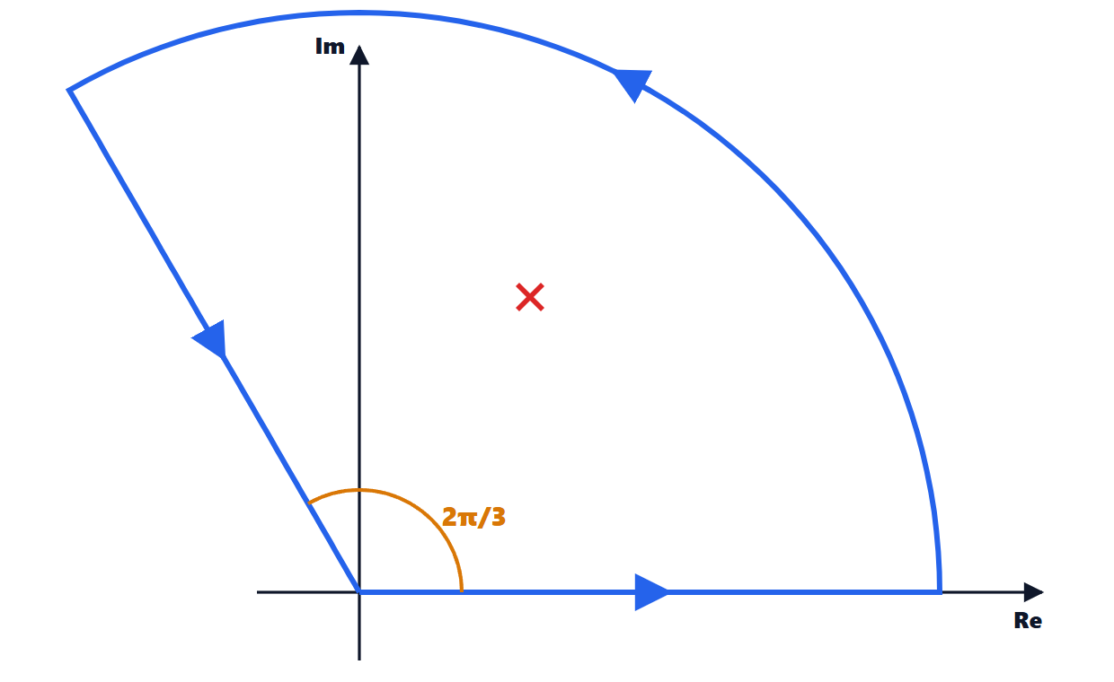
Example.  . The function
 does not change when
 is rotated by
 : integrate over the sector of opening . On the return ray
 ,
 , and that piece equals
 . The arc tends to zero (ML:
 ). Inside there is a single pole,
 , with residue
 . So

(with  and a couple of simplifications).
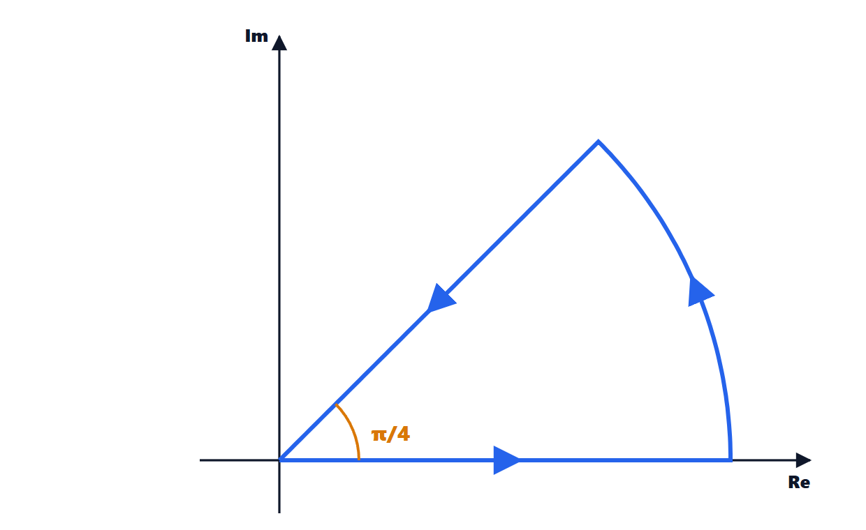
Fresnel integrals. With  and the sector of opening
 : there are no poles inside; on the ray
 ,
 , and the function becomes a Gaussian. The arc tends to zero with the same idea as Jordan (
 ). So
 , and separating real and imaginary parts

These are the integrals of Fresnel diffraction in optics and of the clothoid curve used for road and railway transition curves.
The rectangle: shifting a Gaussian
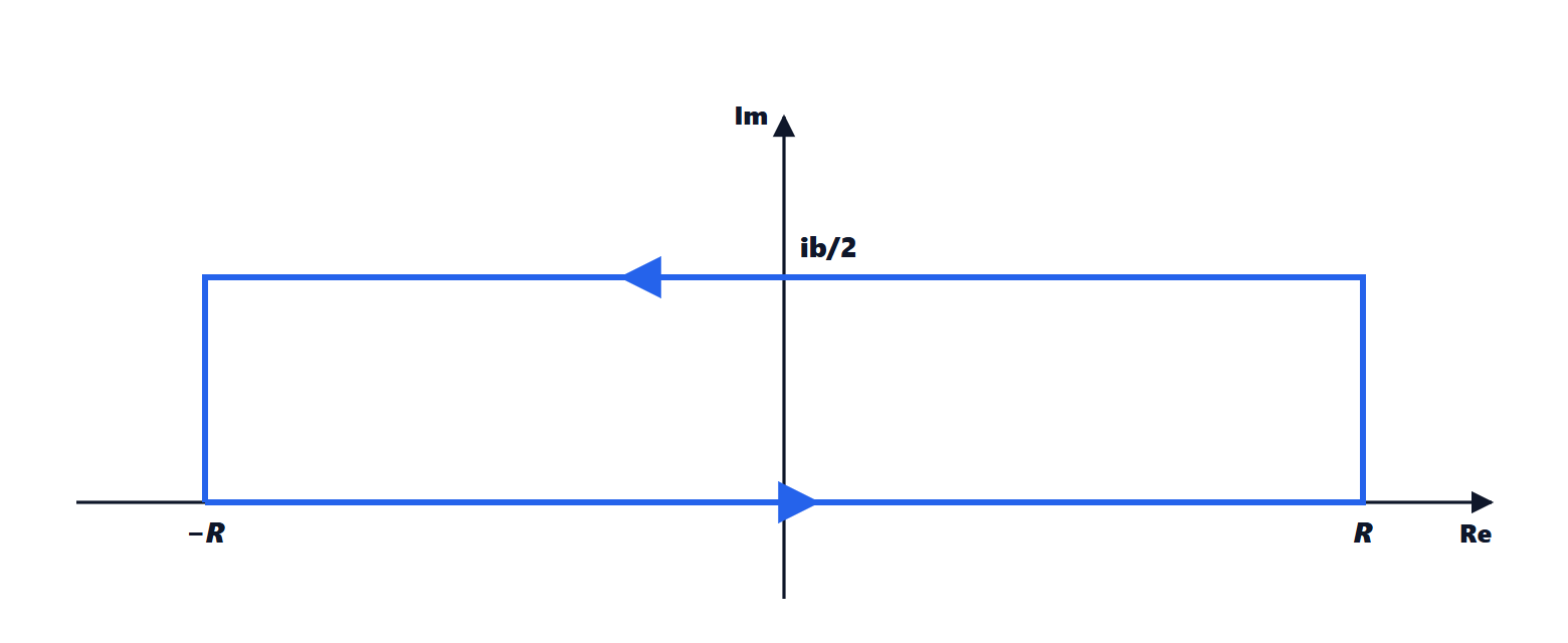
Example.  . Integrate
 , holomorphic everywhere, over the rectangle with vertices
 and
 . On the upper side
 :
 . The vertical sides tend to zero (the integrand is about
 ). So
 , and taking the real part

It is the Fourier transform of the Gaussian, derived in the Fourier transform in-depth study with a differential equation: here with a rectangle.
Trigonometric integrals
With  ,
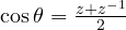 ,
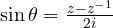 ,
 , an integral over
 becomes an integral over the unit circle (lesson). For a power,
 .
Example.  . The roots of
 are 2 and
 : inside the circle only , with residue
 . Integral:
 .
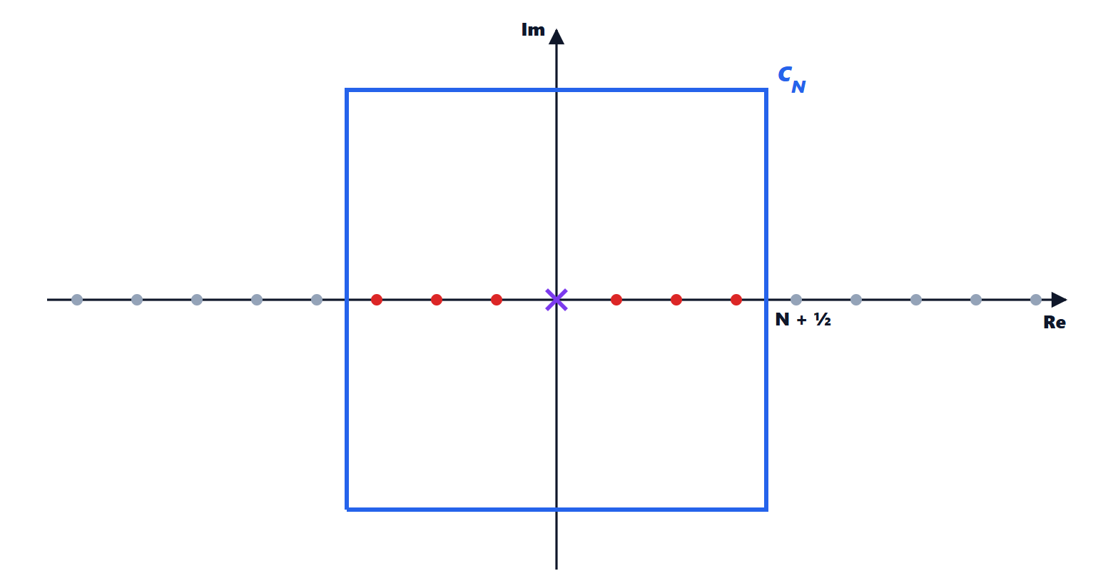
Summing a series with residues
Theorem.  .
Proof. The function  has simple poles at every integer
 , with residue 1. So
 has residue
 at every
 . At 0 the expansion
 gives
 , residue
 . On the square
 with vertices
 , which passes between the integers,
 is bounded by a constant independent of
 ; then
 , the length is about
 , and the integral tends to 0. So the sum of all the residues tends to 0:

∎ This is the Basel problem, solved by Euler in 1734 with another method. With the same idea one sums  and many series of physics.
Exercises with all these contours are on the exercise page linked at the top.