The residue theorem and real integrals
Residues and how to compute them, the residue theorem, integrals on the line with a semicircle, Jordan's lemma, the Dirichlet integral, trigonometric integrals and the argument principle.
The residue theorem is the most used result of complex analysis. It reduces the computation of an integral round a closed curve to the sum of a few numbers, the residues, which are found with derivatives or limits. And it lets you compute real integrals that would be impossible with the methods of Analysis 1: exactly those that appear in Fourier and Laplace transforms.
The residue
The residue of  at an isolated singularity
 is the coefficient
 of the Laurent series, the one of
 :

The equality follows by integrating the Laurent series term by term: from the lesson on Cauchy’s theorem, every term  integrates to zero except
 , which gives
 . The residue is “what is left” after integration.
The residue theorem
Theorem. If is holomorphic inside and on a simple closed curve  , traversed anticlockwise, except at finitely many interior singularities
 , then
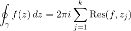
Proof. By Cauchy’s theorem can be deformed into small circles, one around each singularity (as in the figure of the lesson on Cauchy’s theorem). The integral round each is times the corresponding residue.
Computing residues
- Simple pole:
 .
- Simple pole of a ratio
 , with
 ,
 ,
 :
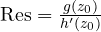 . The handiest formula.
- Pole of order
 :

- Essential singularity: write the Laurent series and read off .
Examples.  at
 :
 .
 at 0: triple pole,
 .
 at 0: from the series
 , the residue is 1.
Real integrals with a semicircle
We want 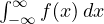 . The idea is to close the segment
 with a semicircle
 in the upper half-plane, apply the residue theorem and show that the integral over the semicircle tends to zero.
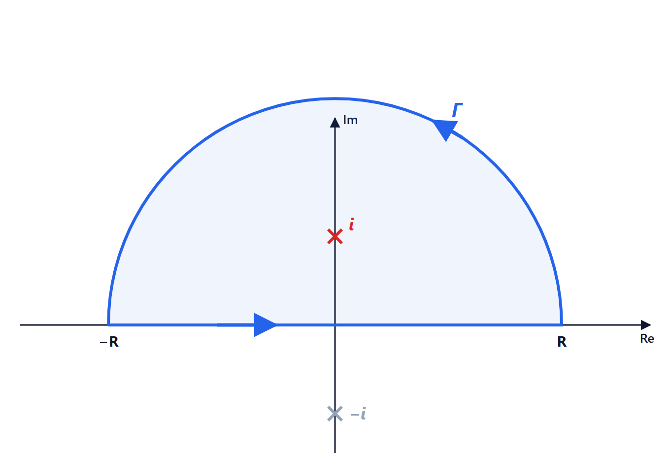
Example.
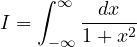
The function  has poles at
 ; only
 is inside the contour, with residue
 . On the semicircle
 and the length is
 , so the semicircle integral is at most
 . What remains is
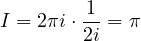
The same result comes from the arctangent, but the method also works when the antiderivative is unknown. General rule: if  is rational, with no poles on the real axis and the degree of
 at least two more than the degree of
 , the semicircle integral tends to zero and

Jordan’s lemma and Fourier integrals
For integrals like  , which are Fourier transforms, the condition is weaker: with
 it is enough that
 on the upper semicircle (Jordan’s lemma), because
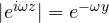 is small where
 .
Example.  . Residue of
 at :
 . So the integral is
 .
The Dirichlet integral. With a small semicircle to go round the pole at the origin one gets
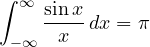
It is the area under the sinc function, which we will meet again as the Fourier transform of the rectangular pulse.
Trigonometric integrals
Integrals  become integrals round the unit circle with
 ,
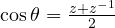 ,
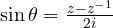 ,
 .
Example.  . The roots of the denominator are
 ; only
 is inside the unit circle. The residue of
 is
 , so the integral is
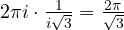 .
The argument principle
One last application, essential in control engineering: for a function with zeros and poles,  , the number of zeros minus the number of poles inside the curve. Geometrically it is the number of times the image
 winds round the origin. The Nyquist criterion uses exactly this to decide whether a feedback system is stable, looking only at the open-loop frequency response.