Solved residue theorem exercises: real integrals computed in the complex plane
Twelve exercises with solutions and graphs: simple and double poles, Fourier integrals, Jordan's lemma, trigonometric integrals, indentation, keyhole, sector, rectangle, summing a series, choosing the contour.
Exercises on the residue theorem applied to real integrals: one starts from an integral on the real line, moves to the complex plane, uses residues and returns to the real line with the result. They are of the kind set in Mathematical Methods courses, in three levels: basic, with rational functions and the semicircle; intermediate, with Jordan’s lemma, trigonometric integrals and the indented contour; exam, with the keyhole, the sector, the rectangle and the summation of a series. The result is given straight away; the full solution, with the graph of the integrand or the contour, opens with a click. The techniques are proved in the in-depth study linked at the top.
Basic level
Exercise 1. Two simple poles in the upper half-plane
Compute 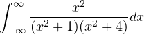 .
Result:  .
Solution
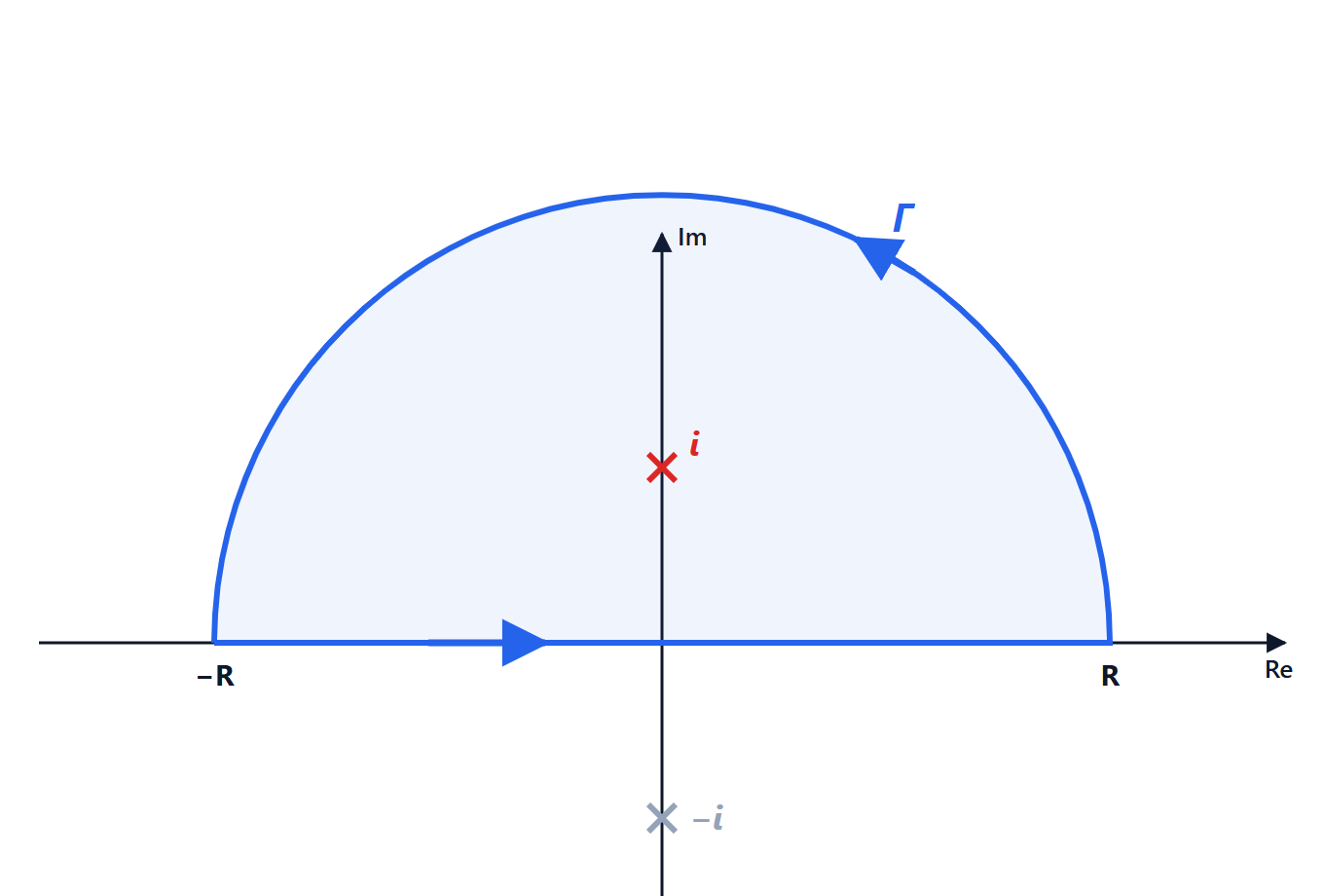
The denominator has degree 2 more than the numerator: close with the upper semicircle. Poles in the upper half-plane:  and
 .
 ;
 .
Sum  ; integral
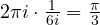 .
Check with partial fractions:  , with integrals
 .
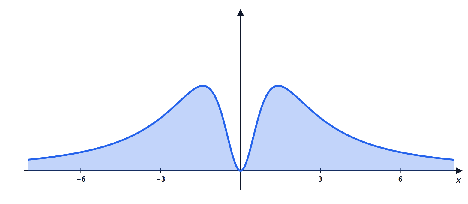
Exercise 2. A double pole
Compute  .
Result:  .
Solution
At  there is a double pole:
 . The residue of a double pole is the derivative of the rest:
 .
Integral:  .
With Calculus 1 one needs the substitution  :
 between
 and , which gives the same .
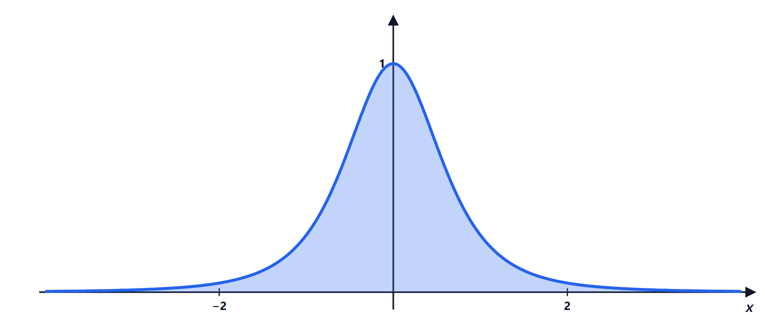
Exercise 3. An irreducible trinomial
Compute 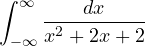 .
Result:  .
Solution
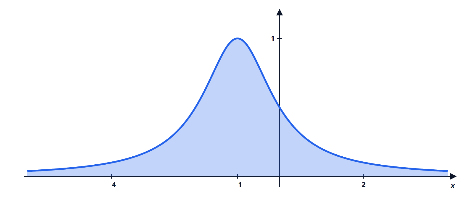
Roots  ; in the upper half-plane
 , with residue
 . Integral:
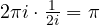 .
As expected:  , and a shift does not change the area of
 .
Intermediate level
Exercise 4. A Fourier integral
Compute 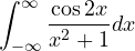 .
Result:  .
Solution
Use 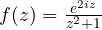 , which is small in the upper half-plane (
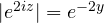 ). Residue at :
 . Integral of
 :
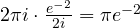 . The result is real, so it is the integral of the cosine.
Beware: with  it would not work, because
 grows exponentially in both directions of the imaginary axis and the arc does not tend to zero.

Exercise 5. When Jordan’s lemma is needed
Compute 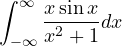 .
Result:  .
Solution
With 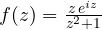 , its imaginary part on the real axis is the integrand. Here
 decays only like
 : the ML estimate would give
 , which does not tend to zero. Jordan’s lemma is needed, with
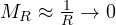 : the arc tends to zero.
Residue at :  . Integral of :
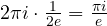 . Imaginary part:
 .
The integral converges only as an improper integral (the integrand decays like  , not absolutely): exactly the case in which Jordan is indispensable.

Exercise 6. A trigonometric integral
Compute 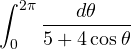 and, in general,
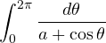 for
 .
Result:  ; in general
 .
Solution
With  :
 . Roots
 and
 : inside the circle only . Residue:
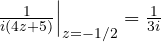 . Integral:
 .
In general,  becomes
 , with roots
 , inside only
 . Residue
 , integral . With
 and the factor 4:
 , consistent. (The lesson has the example
 :
 .)

Exercise 7. The squared sine integral
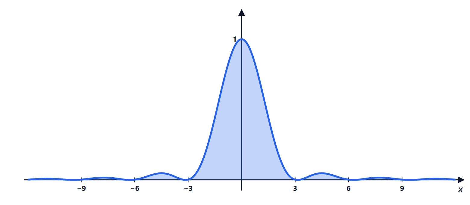
Compute 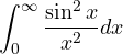 .
Result: .
Solution
 , so the integral over the whole line is
 , the real part of
 with
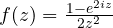 .
has a simple pole at 0 ( , so
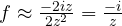 ), with residue
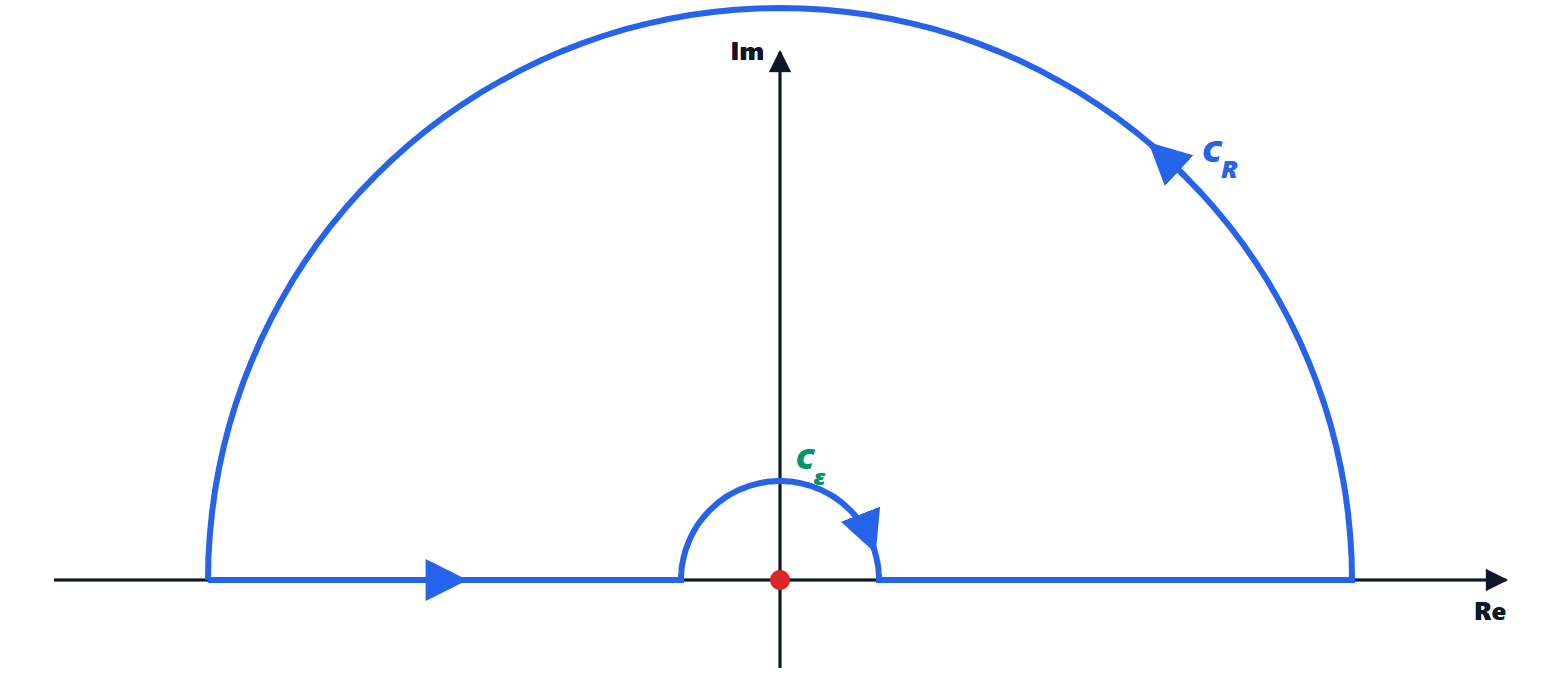
 . Indented contour (in-depth study): no poles inside, the large arc tends to zero (Jordan, with
 and
 ), the small semicircle gives
 . So the integral on the real stretches tends to , and
 .
By symmetry  . The same result follows from Parseval’s theorem (Fourier transform exercises).
Exam level
Exercise 8. The keyhole with a equal to one third
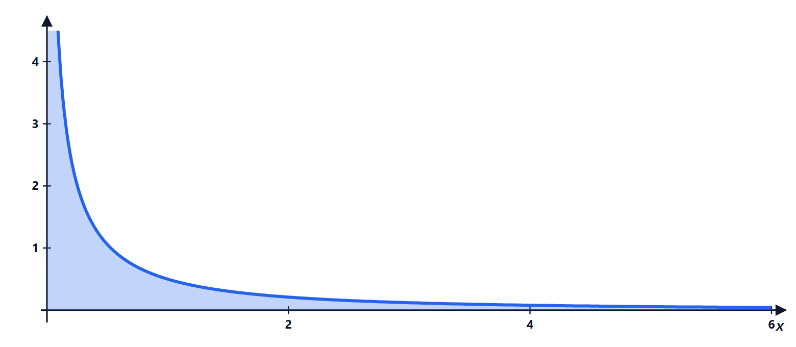
Compute  .
Result:  .
Solution
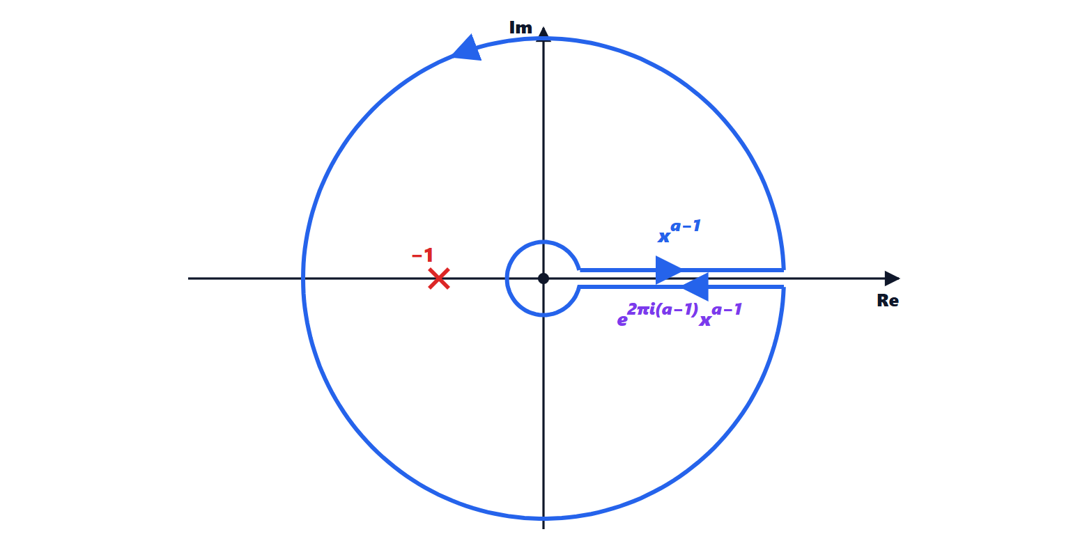
It is the formula of the in-depth study  with
 , i.e.
 :
 .
Redoing the computation: on the lower edge of the cut  ; residue at
 :
 . So
 ,
 . ✓
The circles do not contribute because  : the integrand is integrable both near 0 (
 ) and at infinity (
 ).
Exercise 9. The sector for the fourth power
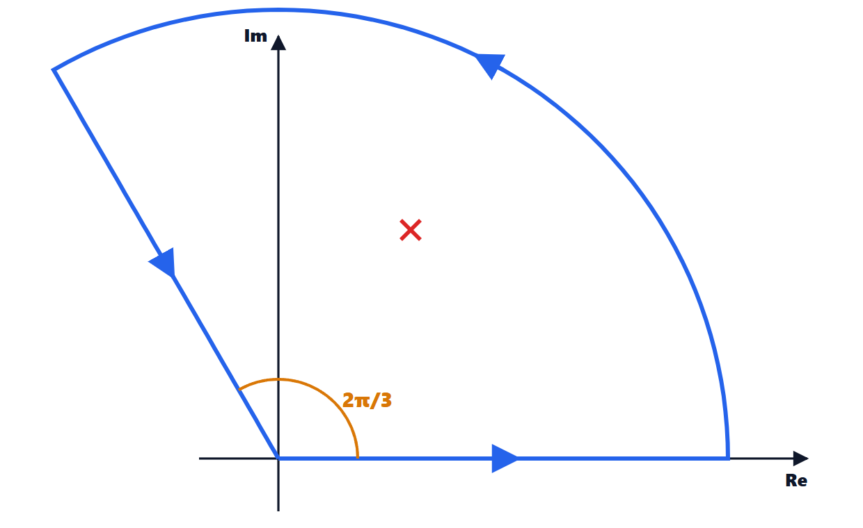
Compute  with a sector of opening .
Result: 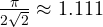 .
Solution
Rotating by ,  does not change: on the ray
 we have
 and
 , so that piece, traversed towards the origin, equals
 . The arc tends to zero (ML). Inside the sector there is a single pole,
 , with residue
 .
 . With
 and
 :
 .
It is half of the integral over the whole line,  , computed in the in-depth study with the semicircle: two different contours, same result.
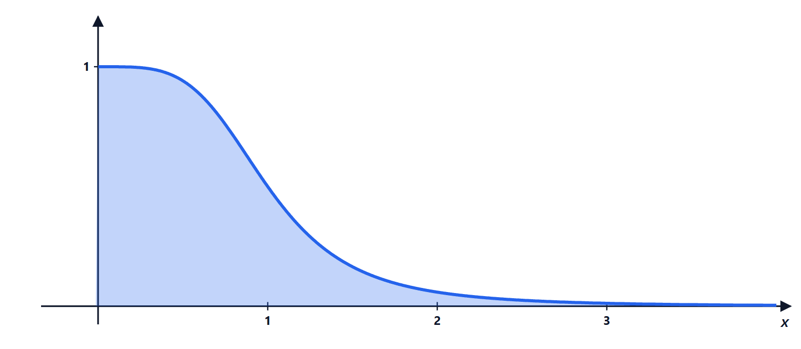
Exercise 10. A modulated Gaussian
Compute  .
Result:  .
Solution
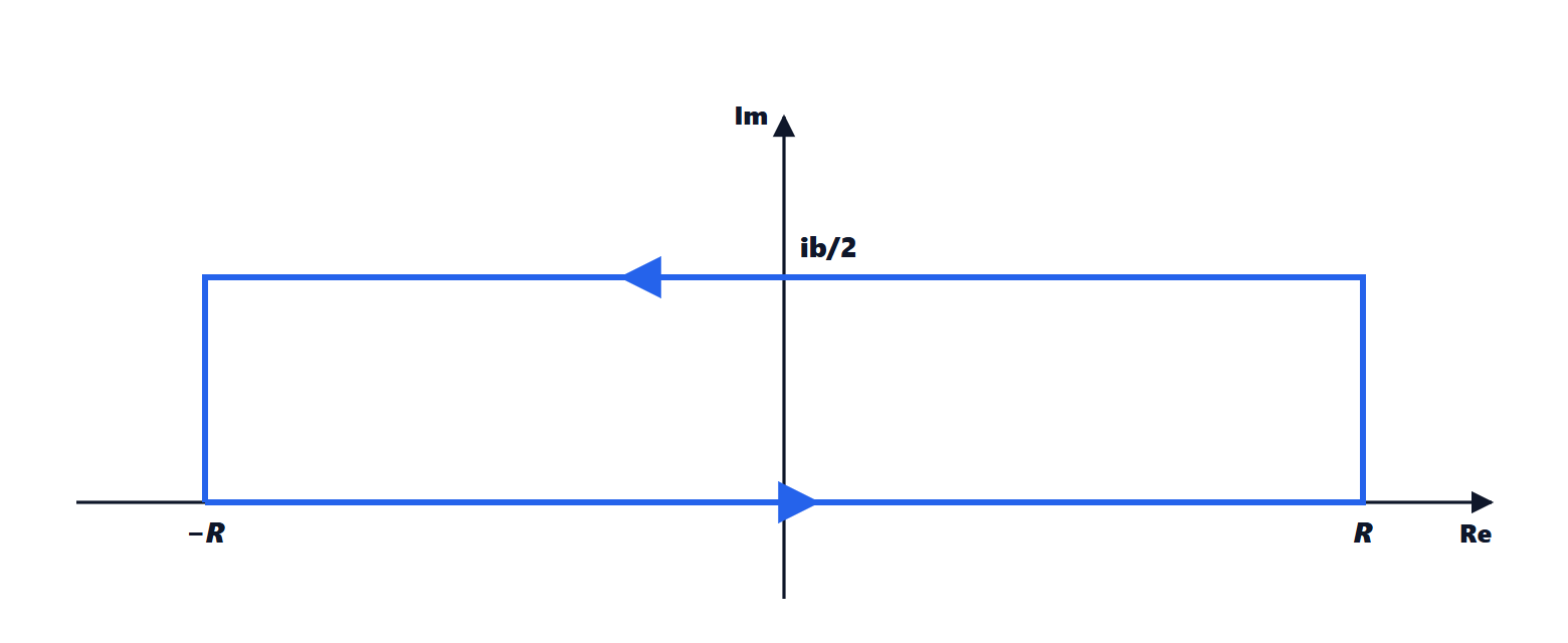
With the rectangle of the in-depth study and  : the height is
 , and on the upper side
 . Cauchy’s theorem (no poles) and the vertical sides tending to zero give
 , i.e.
 (the sine part vanishes by symmetry).
General formula:  . With
 one gets back the Gaussian integral
 .

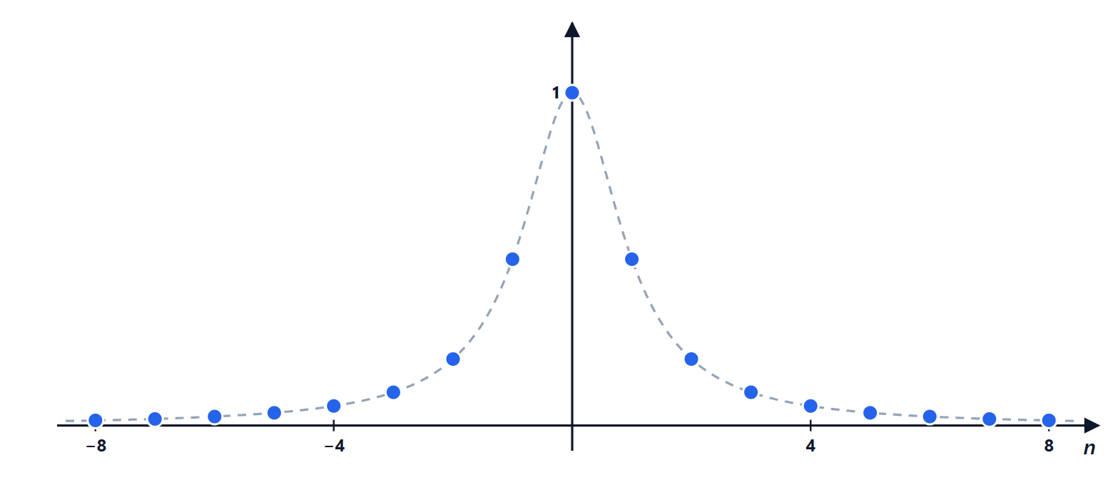
Exercise 11. Summing a series with the hyperbolic cotangent
Compute  .
Result:  .
Solution
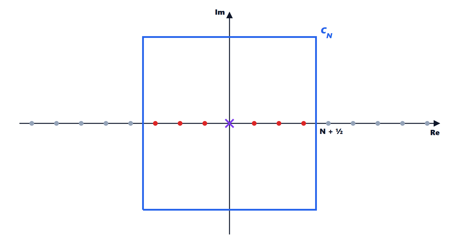
As in the in-depth study, use  : at every integer
 it has residue
 . The other poles are
 :

With  and
 odd: both residues equal
 , in total
 .
On the square  the integral tends to 0, so the sum of all residues is 0:
 . Removing
 and dividing by 2:
 .
Exercise 12. Summary: which contour?
For each of the following integrals state the complex function and the contour to use, without computing them: (a)  ; (b)
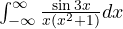 ; (c)
 ; (d)
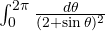 ; (e)
 .
Result: (a) semicircle; (b)  with indentation and Jordan; (c) keyhole; (d) unit circle with ; (e) sector of opening
 .
Solution
(a) Rational function with denominator 6 degrees higher: semicircle, poles  , ,
 . Result .
(b) Simple pole on the real axis (at 0) and slow decay: use , indented contour around 0, Jordan for the large arc, pole inside. Result  .
(c) Non-integer power: cut along the positive half-axis, keyhole (or the formula for  ). Result .
(d) Trigonometric integral over one period: , 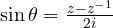 ; it becomes a double pole inside the circle. Result
 .
(e)  is invariant under rotations by : a sector with that opening, a single pole
 . Result
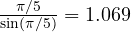 .
Choosing the contour is half the exercise: it depends on where the poles are, on how the integrand decays and on the symmetries.