Ohm's law from the structure of matter: the Drude model
Current density from the carriers, conductivity derived from electron collisions with the lattice, the numbers for copper, Joule heating, resistance of conductors of any shape, temperature dependence, limits of Ohm's law and the Hall effect.
This page goes deeper into the lesson on electric current: it derives Ohm’s law from the microscopic properties of matter, that is, from the free electrons of a metal colliding with the crystal lattice. This is the Drude model (1900). From a simple idea we obtain the conductivity in terms of atomic quantities, the numerical value of the time between collisions in copper, Joule heating seen as energy given to the lattice, the temperature dependence, the resistance of conductors of any shape, the limits of validity of the law and the Hall effect, which allows the number and sign of the carriers to be measured.
Current density from the carriers
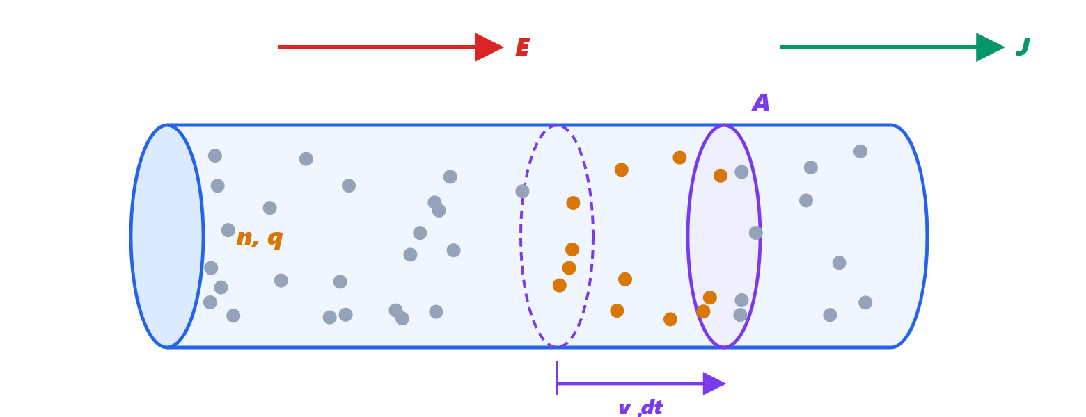
Theorem. If a conductor contains  carriers per unit volume, each with charge
 and mean (drift) velocity
 , the current density is

Proof. Consider a cross-section of area  perpendicular to . In a time
 it is crossed by all the carriers lying within a distance
 upstream, that is, those contained in the cylinder of volume
 . There are
 of them, and they carry the charge
 . The current is
 , and the density
 . ∎
For electrons  : is opposite to
 , but the product
 has the direction of the conventional current.
The Drude model
There are four assumptions, all simple:
- in the metal some of the electrons (one or two per atom) are free to move, like a gas, among the fixed ions of the lattice;
- between collisions an electron moves under the action of external forces only, here
 ;
- collisions are instantaneous, and after each collision the velocity has a random direction: on average, just after a collision, the velocity is zero;
- the probability of a collision in an interval is
 , independent of the electron’s history.
 is called the relaxation time or mean time between collisions.

Theorem. In the Drude model the drift velocity and the conductivity are

Proof. Look at one electron at a given instant. A time  has passed since its last collision, and during that time the field has accelerated it with
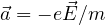 . Its velocity is therefore
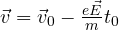 , where
 is the velocity just after the collision.
Average over all the electrons. By assumption 3, the average of is zero. By assumption 4, the time elapsed since the last collision has an exponential distribution with mean (the probability that no collision has occurred in the last seconds is  ). Hence

Substituting into 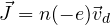 :
 . ∎
Another way to see it. On average, the force of the field and the effect of collisions balance: collisions behave like viscous friction, which every second destroys a fraction  of the ordered momentum. The equation of the average motion is
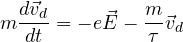
At steady state  and the same result follows. The transient lasts a few , about
 s: for every practical purpose the current follows the field instantly.
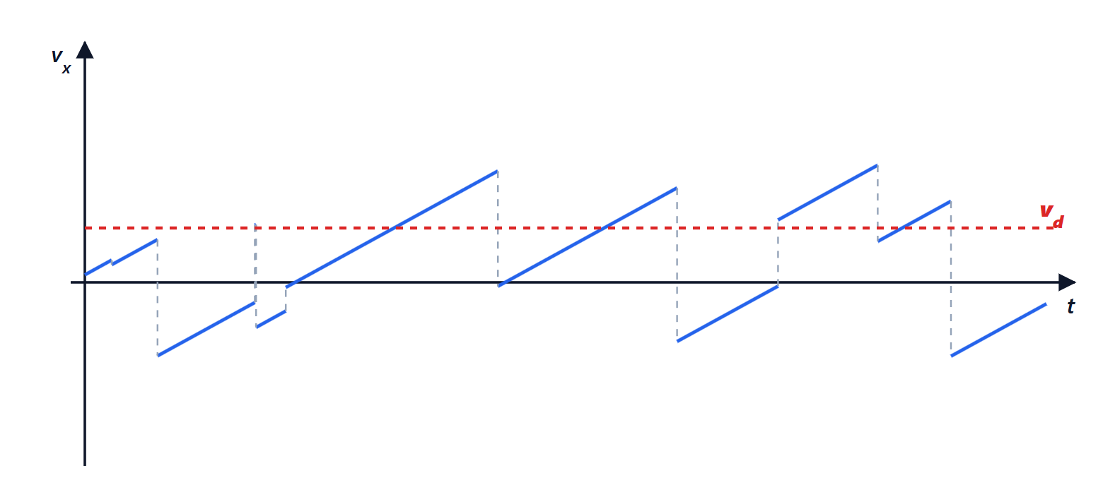
Ohm’s law is therefore the consequence of one fact: collisions make the electron “forget” the velocity it has gained, and the average velocity stays proportional to the field instead of growing without limit. In a conductor without collisions ( ) the current would grow indefinitely under a constant field: that is what happens in the vacuum of a cathode-ray tube, not in a wire.
The numbers for copper
The time between collisions can be obtained from the measured resistivity. For copper  Ω·m and
 m
 (one free electron per atom):

Three comparisons show the scales.
Drift versus thermal motion. In a 1 mm² wire carrying 1 A the field is  V/m and the drift velocity
 m/s, the same value found in the lesson from
 . The electrons, on the other hand, move randomly at speeds of order
 m/s: the drift is a tiny correction to a very fast disordered motion.
The mean free path. With the “classical” thermal speed  m/s at 300 K, the distance between collisions would be
 nm, about ten interatomic distances: consistent with Drude’s picture of electrons hitting the ions. But quantum mechanics says that conduction electrons move at the Fermi velocity,
 m/s in copper, and then
 nm, about 150 interatomic distances.
The role of the ions. An electron thus travels past hundreds of atoms without colliding: a perfectly regular lattice does not scatter electrons (a result of quantum mechanics, linked to the wave nature of the electron). Collisions happen with the imperfections of the lattice: thermal vibrations of the ions (phonons), impurities, defects, grain boundaries. The Drude model has the wrong picture of collisions but the right structure of the formula: with the right effective mass and relaxation time,  remains valid in the quantum theory too.
Joule heating seen from the lattice
Theorem. In an ohmic conductor the power dissipated per unit volume is
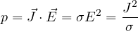
and integrated over a wire it gives  .
Proof. On each carrier the field does work at a rate  . On average, per unit volume,
 . At steady state the average kinetic energy of the electrons does not grow: all this energy is given to the lattice in collisions, and becomes thermal agitation of the ions, that is, heat. In a wire of cross-section and length
 with uniform field,
 . ∎
The resistance of a conductor of any shape
From the local law  the resistance of an object follows by integration. For a uniform wire,
 and
 give
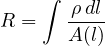
 . If the cross-section changes along the current path, divide the conductor into slices of thickness
 in series, each with resistance
 :
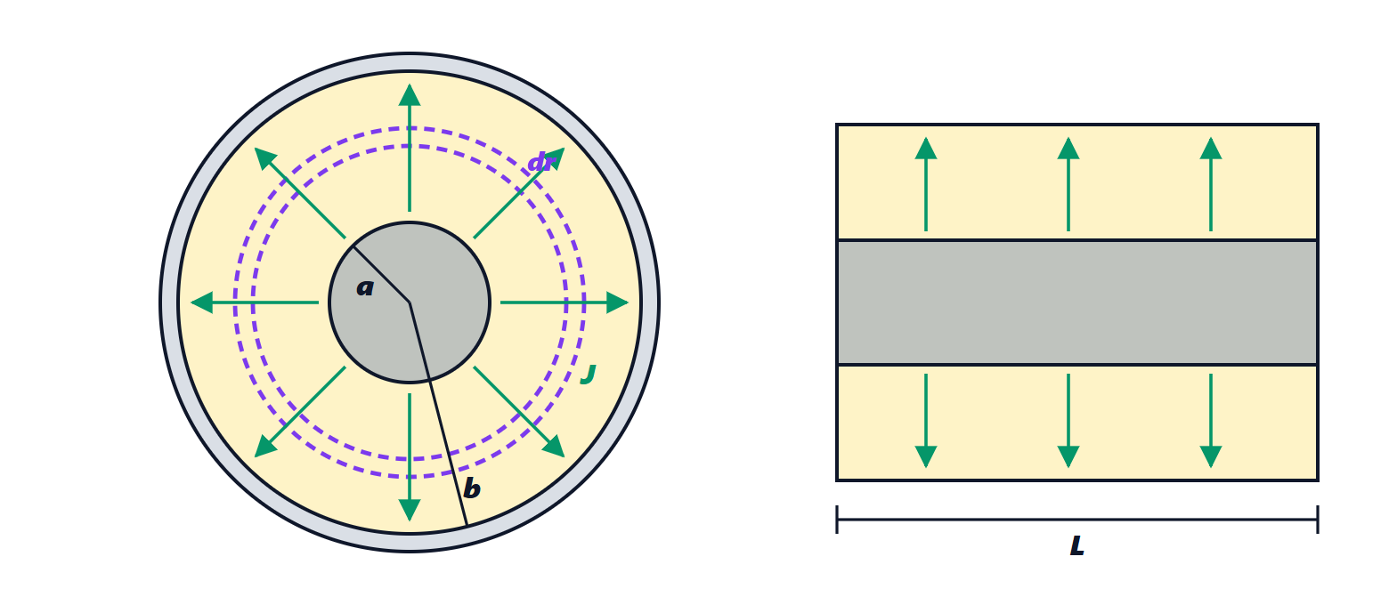
Example: leakage through the insulation of a coaxial cable. Between the inner conductor (radius  ) and the braid (radius
 ) there is an insulator of very large resistivity
 , of length . The leakage current flows radially, through cylindrical shells of radius
 , thickness
 and area
 , all in series:

The resistance decreases with length, unlike a wire: a longer cable has more surface through which to leak current. With  Ω·m (polyethylene),
 and
 m:
 Ω.
Temperature dependence
In metals does not depend on temperature; does. Collisions with lattice vibrations are more frequent the more the ions vibrate, and the mean square amplitude of the vibrations is proportional to  (above a few tens of kelvin). So
 and the resistivity grows linearly. Collisions with impurities, instead, do not depend on . The two causes add up (Matthiessen’s rule):

where  is the residual resistivity at very low temperature, which measures the purity of the metal. For copper
 K
 .
In semiconductors the story is the opposite: the number of carriers grows exponentially with temperature,  , because thermal agitation frees electrons from the bonds. The increase of outweighs the decrease of , and the resistivity decreases rapidly as rises. This is the reason for NTC thermistors.

When Ohm’s law does not hold
Proportionality between  and
 requires and not to depend on the field, and the field to vary slowly compared with . Outside these conditions:
- strong fields in semiconductors: the drift velocity saturates (about
 m/s in silicon), because the electrons give energy to the lattice as fast as they receive it;
- high frequencies: with an alternating field of angular frequency
 , the same equation of average motion gives
 (with the phasor convention of electrical engineering). For metals
 up to about
 Hz: the DC Ohm’s law holds for all of electronics, but not for light: at optical frequencies the free-electron model, extended, explains why metals reflect visible light;
- non-linear devices: diodes, transistors, gas discharges, where depends on the applied voltage;
- conductors shorter than the mean free path: in nanowires electrons pass without collisions (ballistic conduction) and the conductance is quantised: each conduction channel contributes
 µS, and a conductor with a single channel has a resistance of about 12.9 kΩ with no collisions at all;
- superconductors: below the critical temperature the resistance is exactly zero.
The Hall effect: counting the carriers
In a strip carrying current and placed in a perpendicular magnetic field  , the Lorentz force
 pushes the carriers towards one edge. Charge accumulates there until the transverse electric field
 that forms balances the magnetic force:
 .
Theorem. In a strip of thickness  (in the direction of ), the Hall voltage is

and its sign depends on the sign of the carriers.
Proof. With width  ,
 . From the current,
 , so
 . Substituting,
 . If the carriers are negative, for the same current direction they move the opposite way, but their charge is also opposite: the Lorentz force pushes them onto the same edge as positive carriers, and the voltage changes sign. ∎
Example. A copper strip 0.1 mm thick carrying 1 A in a 1 T field:  µV. In semiconductors is a million times smaller and
 becomes tens of millivolts: this is the principle of Hall sensors, used to measure magnetic fields and currents without contact.

Historically the Hall effect showed that in some metals, such as zinc, the carriers behave like positive charges (holes): a fact the Drude model could not explain and one of the proofs of the quantum theory of solids.
Exercises on resistance, DC circuits and the RC circuit are on the exercise page linked at the top.