Electric current, Ohm's law, Kirchhoff's laws and the RC circuit
Current and drift velocity, resistivity, Joule heating, sources and Kirchhoff's laws, capacitor charging with proof and the energy balance.
So far charges have been at rest. When they move there is an electric current, and with currents come circuits. This lesson is the bridge between physics and circuit theory: it defines current and resistance starting from the motion of electrons, derives Ohm’s law and Joule heating, introduces Kirchhoff’s laws and studies the RC circuit.
Electric current
Current is the charge crossing a section of the conductor per unit time:
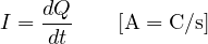
By convention its direction is the one in which positive charges would move; in metals electrons move the opposite way. The current density  (A/m²) is the current per unit area.
Drift velocity
If the conductor has  carriers per unit volume, each with charge
 , moving on average with velocity
 , then
 .
Example. A 1 mm² copper wire carrying 1 A. Copper has about  free electrons per m³.
 m/s: less than a tenth of a millimetre per second. A lamp lights up at once not because electrons race along, but because the field travels along the wire at nearly the speed of light and sets all the electrons in the circuit moving at the same time.
Ohm’s law and resistivity
In many materials current density is proportional to the field:  , with
 the conductivity. For a wire of length
 and cross-section
 , with
 and
 :
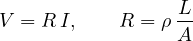
where  is the resistivity (Ω·m). Copper has
 Ω·m: one metre of 1 mm² wire has 17 mΩ. A printed circuit trace 0.25 mm wide in 35 µm copper has about 2 mΩ per millimetre, and a 10 cm trace carrying 2 A drops 0.4 V: enough to upset a precision circuit.
The resistivity of metals rises with temperature (for copper about 0.4% per degree), that of semiconductors falls. The first effect is used in platinum temperature sensors (Pt100), the second in NTC thermistors.
Power and Joule heating
A charge  crossing a potential difference
 gives up energy
 . The power is
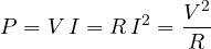
In resistors this energy becomes heat (Joule heating): electrons accelerated by the field collide with the lattice and give up energy. It is the principle of electric heaters and fuses, and the reason power lines work at high voltage: for the same power the current is smaller, and the  losses fall with its square.
Sources and Kirchhoff’s laws
A source maintains a potential difference by spending another form of energy (chemical in a battery, mechanical in a dynamo). Its electromotive force  is the work per unit charge; a real source also has an internal resistance
 , and across its terminals you measure
 .
Kirchhoff’s laws let you analyse any circuit:
- at nodes: the sum of the currents in equals the sum of the currents out (conservation of charge);
- around loops: along any closed path the sum of the voltages is zero (the electrostatic field is conservative).
The rules for connections follow: in series resistances add, in parallel conductances  add.
The RC circuit
A capacitor  charges through a resistance
 from a source .
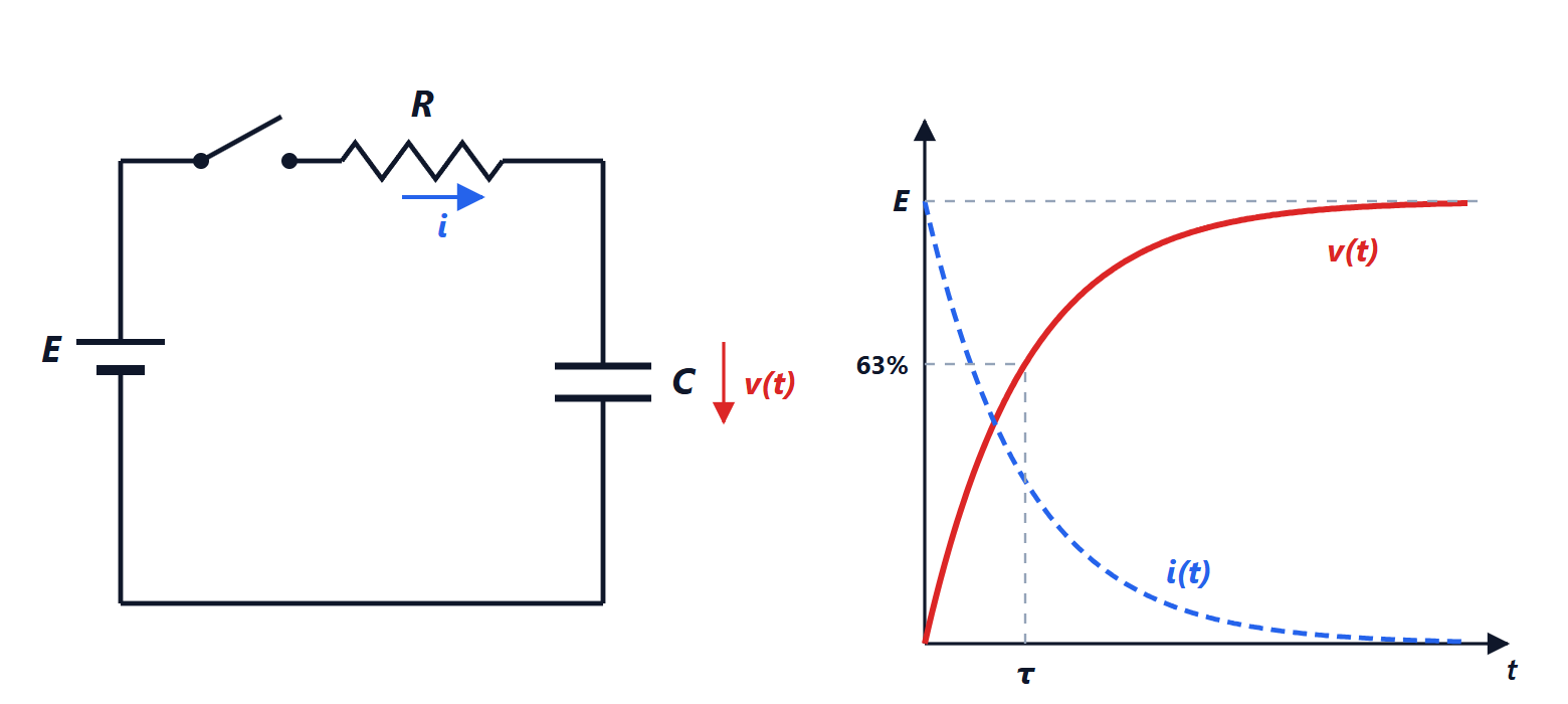
Proof of the charging law
By the loop law,  , with
 and
 :
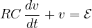
It is a first-order linear equation (Analysis 2 lesson): with the capacitor initially empty,

At the first instant the empty capacitor behaves like a short circuit ( ); in steady state like an open circuit (
 ). The time constant
 measures the speed of the transient: with
 kΩ and
 nF,
 ms, and after
 ms the capacitor is 99.3% charged.
The energy balance
The source supplies a total of  . The capacitor keeps
 . The other half is dissipated in the resistor,
 , whatever the value of . Charging a capacitor from a constant voltage source always wastes half the energy: one reason why digital circuits consume in proportion to
 , and why lowering the supply voltage is the most effective way to cut consumption.
The RC circuit is everywhere: in low-pass and high-pass filters, in microcontroller reset circuits, in timers like the 555 and in push-button debouncing circuits.



