Electric potential and equipotential surfaces
Potential energy and potential, the electronvolt, the field as the gradient of the potential, equipotential surfaces, connected spheres and the dipole, field energy and dielectric strength.
The electric field is a vector, and working with vectors is laborious. Since the electrostatic force is conservative, everything can be described with a single scalar function, the electric potential. Its difference between two points is the voltage, the quantity measured with a voltmeter and reasoned about in every circuit. In this lesson we define the potential and look at its link with the field and at equipotential surfaces.
Electric potential energy
Coulomb’s force is central and depends only on distance, so it is conservative (Analysis 2 lesson on conservative fields): the work to move a charge does not depend on the path. A potential energy can therefore be defined. For two point charges, with zero at infinity:
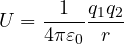
It is positive for like charges (work must be spent to bring them together) and negative for unlike charges (the system is bound).
Electric potential
The potential at a point is the potential energy per unit charge:
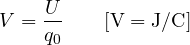
For a point charge  , and for several charges the potentials add up as plain numbers: much simpler than adding vectors.
The potential difference between two points is the work done by the field per unit charge, with the sign changed:
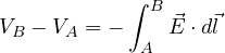
A charge  crossing a potential difference
 gains or loses energy
 . An electron accelerated through 1 V gains
 J, one electronvolt (eV), the energy unit of atomic and semiconductor physics: the band gap of silicon is 1.12 eV.
From potential to field
The integral is inverted by a derivative: the field is minus the gradient of the potential

The field points where the potential decreases fastest. In a uniform field, as between the plates of a parallel-plate capacitor,  : with 10 V across 1 mm the field is 10 kV/m. That is why the unit of field is often written V/m.
Equipotential surfaces
They are the surfaces on which  is constant, the “level curves” of the potential. Since the gradient is perpendicular to level curves:
- field lines are perpendicular to equipotential surfaces;
- moving a charge along an equipotential surface takes no work.
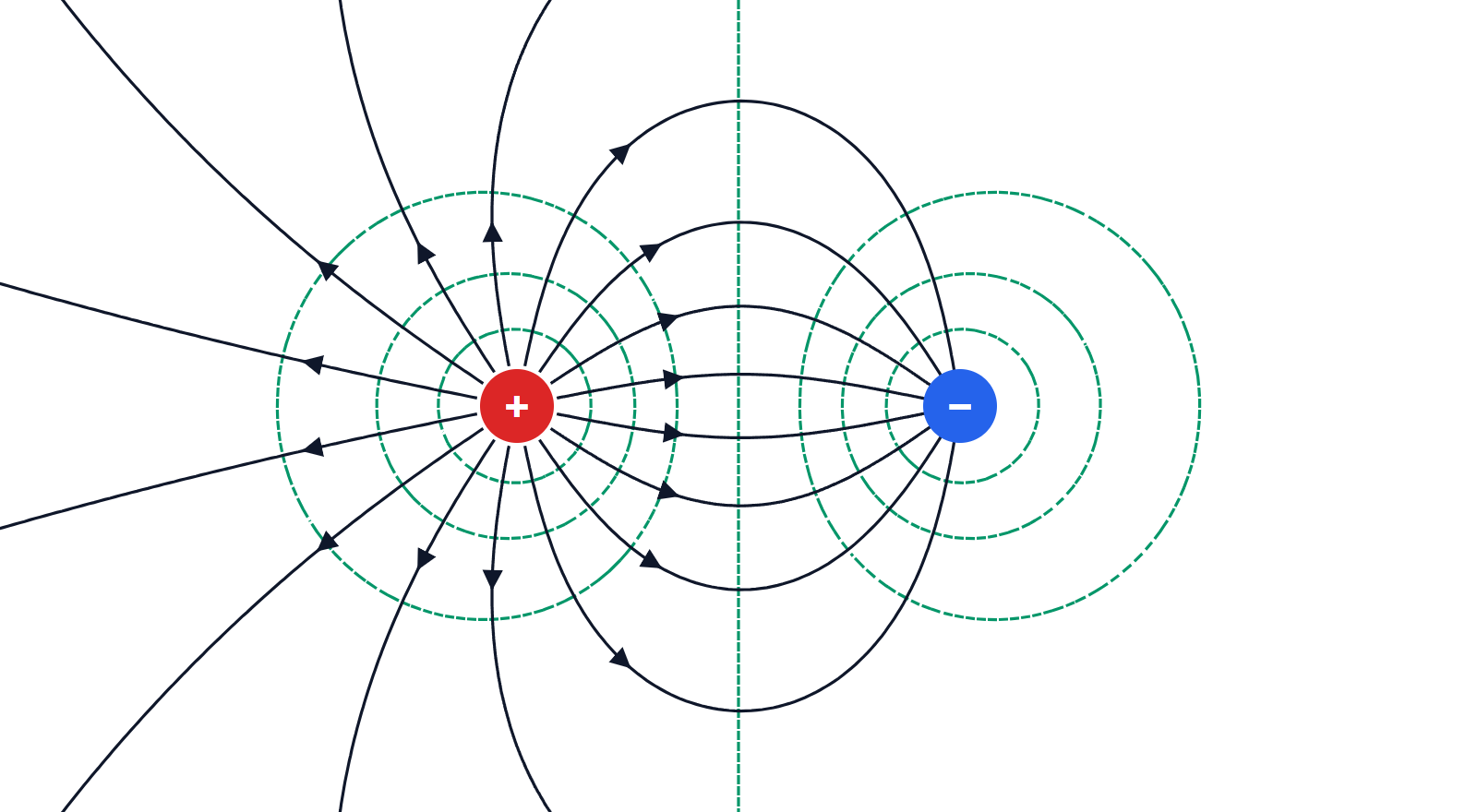
A conductor in equilibrium is all at the same potential: inside it the field is zero, so there are no potential differences. Its surface is an equipotential, which is why the field just outside is perpendicular to the surface.
Worked examples
Conducting sphere with charge  , radius
 : outside the potential is
 ; on the surface and inside it equals
 , constant.
Two spheres joined by a wire. Two conducting spheres of radii  and
 , far apart and joined by a wire, are at the same potential:
 . The surface densities are then in the ratio
 : the smaller sphere has the stronger field. It is the quantitative explanation of the point effect.
The dipole. Two charges  and
 a distance
 apart. At a distance
 , at an angle
 from the axis:

The dipole potential falls as  , faster than that of a single charge, because from far away the two charges nearly cancel. Polar molecules such as water are dipoles, and the properties of dielectrics depend on this.
The energy of a charge distribution
Assembling a system of charges takes work, which is stored as electrostatic energy. The energy can be thought of as located in the field itself, with a density

It is the same result we will find for the energy of a capacitor, and it shows that the field is not just a calculating device: it carries energy, as we will see with electromagnetic waves.
Dielectric strength
Every insulator withstands a maximum field before it starts to conduct (breakdown). For dry air it is about 3 MV/m, that is 3 kV per millimetre. This value sets the creepage and clearance distances on printed circuit boards carrying mains voltage, and the maximum voltage of capacitors and transistors: silicon dioxide withstands about 1 V per nanometre, so the gate oxide of a modern transistor, a few nanometres thick, reaches its limit at a few volts.