Mathematical Methods

Solved Laplace transform exercises: differential equations, circuits and systems

Twelve exercises with solutions and graphs: transforms and inverse transforms, repeated and complex poles, differential equations, piecewise signals, final value, convolution, RLC circuit, second-order system, square wave, integral equation.

ielettronica 25 October 2026 8 min read 0 comments

Exercises on the Laplace transform of the kind set in Mathematical Methods, Circuit Theory and Control courses, in three levels: basic, with direct transforms and inverse transforms; intermediate, with differential equations, delays, final value theorems and convolution; exam, with circuits, second-order systems, periodic signals and integral equations. The result is given straight away; the full solution, with the graph, opens with a click. The tables are in the in-depth study linked at the top.

Basic level

Exercise 1. A power times an exponential

Compute $\mathcal L\{t^2e^{-3t}\}$ .

Result: $\dfrac{2}{(s + 3)^3}$ .

Solution

With the shift in s: $\mathcal L\{t^2\} = \frac{2}{s^3}$ , and multiplying by $e^{-3t}$ replaces $s$ with $s + 3$ : $\frac{2}{(s + 3)^3}$ .

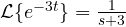
With the derivative: from $\mathcal L\{e^{-3t}\} = \frac{1}{s + 3}$ and $\mathcal L\{t^2f\} = F''(s)$ : $\frac{d^2}{ds^2}\frac{1}{s + 3} = \frac{2}{(s + 3)^3}$ .

The result has a triple pole at $-3$ : this is the kind of term that appears when a system has coincident poles.

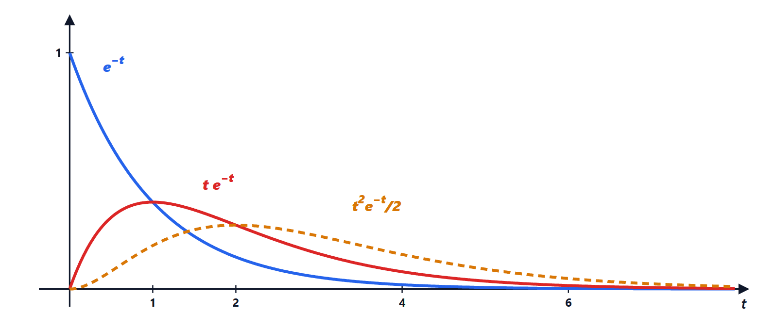
Responses of repeated poles — Simple, double and triple poles produce terms e to the minus t multiplied by increasing powers of t.

Exercise 2. The square of sine

Compute $\mathcal L\{\sin^2 t\}$ .

Result: $\dfrac{2}{s(s^2 + 4)}$ .

Solution

$\sin^2 t = \frac{1 - \cos 2t}{2}$ , so

$\mathcal L\{\sin^2 t\} = \frac{1}{2}\left(\frac{1}{s} - \frac{s}{s^2 + 4}\right) = \frac{1}{2}\cdot\frac{s^2 + 4 - s^2}{s(s^2 + 4)} = \frac{2}{s(s^2 + 4)}$

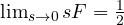
Check with the initial value: $\lim_{s\to\infty}sF = 0 = \sin^2 0$ . The final value theorem cannot be used: the poles $\pm 2i$ lie on the imaginary axis and the function oscillates.

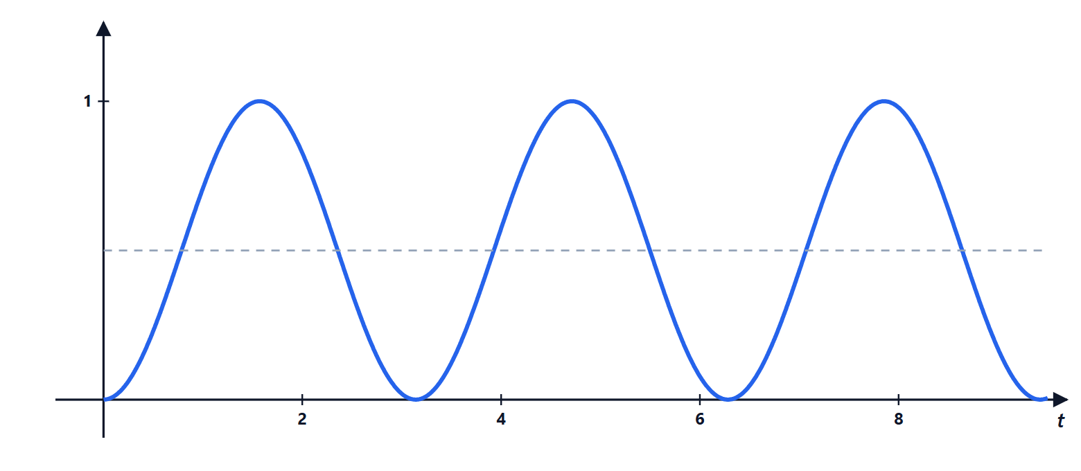
The square of sine — The function oscillates between 0 and 1 around the mean value one half, dashed, without tending to a limit.

Exercise 3. A double pole at the origin

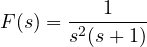
Find the inverse transform of $F(s) = \dfrac{1}{s^2(s + 1)}$ .

Result: $f(t) = t - 1 + e^{-t}$ .

Solution

Partial fractions: $\dfrac{1}{s^2(s + 1)} = \dfrac{A}{s} + \dfrac{B}{s^2} + \dfrac{C}{s + 1}$ .

$C$ : cover $s + 1$ and set $s = -1$ : $C = \frac{1}{1} = 1$ . $B$ : cover $s^2$ and set $s = 0$ : $B = 1$ . $A$ : it is the derivative of $\frac{1}{s + 1}$ at $s = 0$ , i.e. $-1$ (or from the coefficient of $s^2$ : $0 = A + C$ ).

Inverting term by term: $f(t) = -1 + t + e^{-t}$ .

Checks: $f(0) = 0$ , $f'(0) = 1 - 1 = 0$ , consistent with $F \sim 1/s^3$ for large $s$ . For large $t$ , $f \approx t - 1$ : a delayed ramp, the response of a first-order system to a ramp.

The function t minus 1 plus e to the minus t — The curve starts from zero with a horizontal tangent and approaches the line t minus 1, dashed.

Exercise 4. Complex conjugate poles

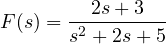
Find the inverse transform of $F(s) = \dfrac{2s + 3}{s^2 + 2s + 5}$ .

Result: $f(t) = e^{-t}\left(2\cos 2t + \frac{1}{2}\sin 2t\right)$ .

Solution

The denominator has $\Delta \lt 0$ : poles $-1 \pm 2i$ . Complete the square: $s^2 + 2s + 5 = (s + 1)^2 + 4$ .

Rewrite the numerator in terms of $s + 1$ : $2s + 3 = 2(s + 1) + 1$ .

$F = 2\,\frac{s + 1}{(s + 1)^2 + 4} + \frac{1}{2}\cdot\frac{2}{(s + 1)^2 + 4} \;\leftrightarrow\; 2e^{-t}\cos 2t + \frac{1}{2}e^{-t}\sin 2t$

The real part of the poles ( $-1$ ) gives the damping, the imaginary part (2) the angular frequency.

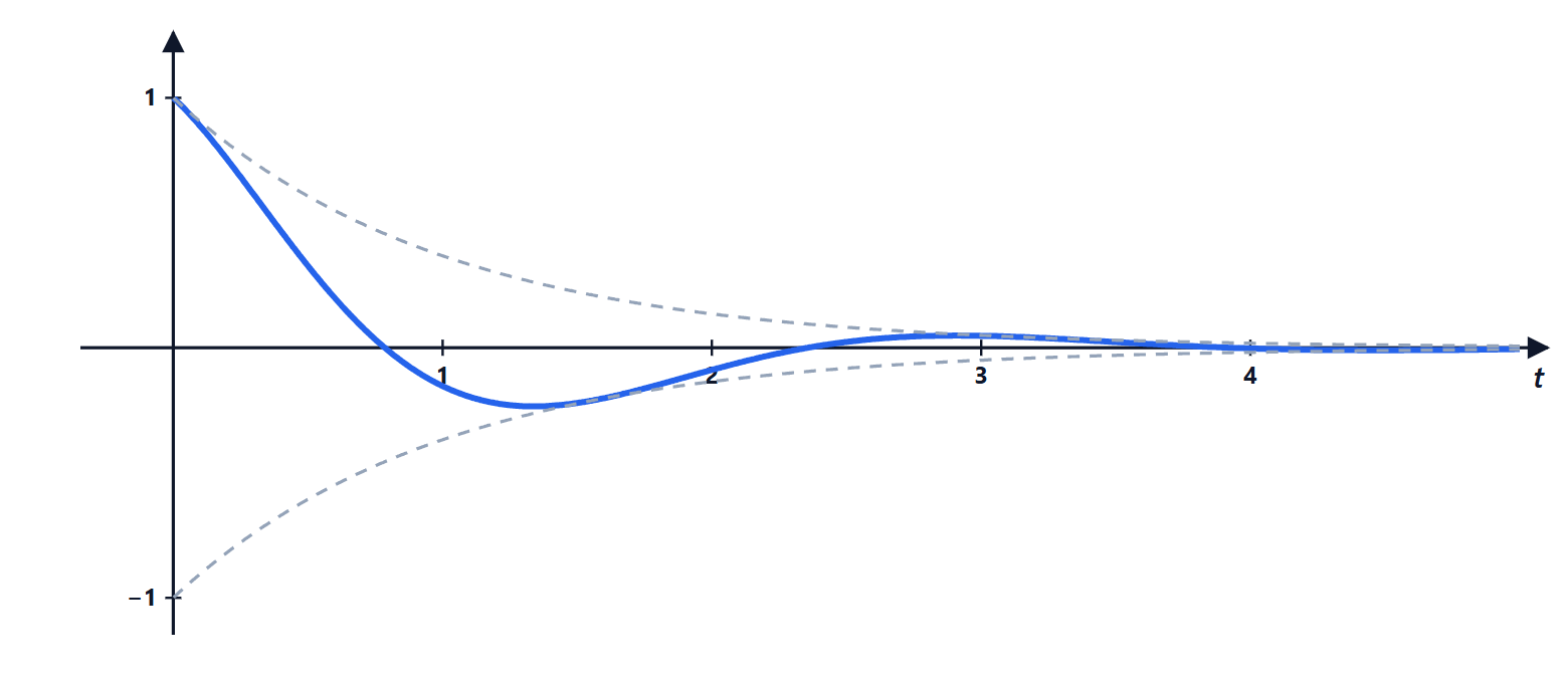
Damped oscillation — A pair of complex poles with real part minus 1 and imaginary part 2 produces an oscillation of angular frequency 2 inside an exponential envelope.

Intermediate level

Exercise 5. A differential equation with initial conditions

Solve $y'' + 3y' + 2y = 1$ for $t \ge 0$ , with $y(0) = 1$ and $y'(0) = 0$ .

Result: $y(t) = \frac{1}{2} + e^{-t} - \frac{1}{2}e^{-2t}$ .

Solution

Transforming, with the initial conditions entering by themselves:

$s^2Y - s\cdot 1 - 0 + 3(sY - 1) + 2Y = \frac{1}{s}$

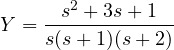
$Y(s^2 + 3s + 2) = \frac{1}{s} + s + 3$ , so $Y = \dfrac{s^2 + 3s + 1}{s(s + 1)(s + 2)}$ .

Residues (Heaviside’s rule): at $s = 0$ : $\frac{1}{2}$ ; at $s = -1$ : $\frac{1 - 3 + 1}{(-1)(1)} = 1$ ; at $s = -2$ : $\frac{4 - 6 + 1}{(-2)(-1)} = -\frac{1}{2}$ .

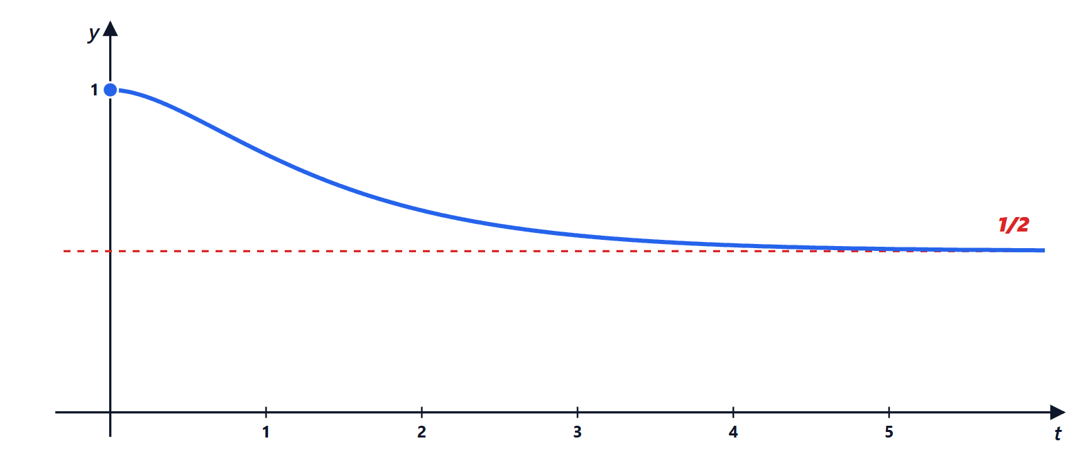
$y(t) = \frac{1}{2} + e^{-t} - \frac{1}{2}e^{-2t}$ . Checks: $y(0) = 1$ , $y'(0) = -1 + 1 = 0$ , $y(\infty) = \frac{1}{2}$ (with the final value theorem: $\lim sY = \frac{1}{2}$ , allowed because the poles of $sY$ are $-1$ and $-2$ ).

Compared with the classical method (homogeneous plus particular plus constants) no system for the constants has to be solved: the initial conditions are already inside $Y$ .

Solution of the differential equation — The solution starts from 1 with a horizontal tangent and falls towards the steady-state value one half.

Exercise 6. A piecewise signal

Find the transform of $f(t) = t$ for $0 \le t \lt 1$ and $f(t) = 1$ for $t \ge 1$ (a saturating ramp).

Result: $F(s) = \dfrac{1 - e^{-s}}{s^2}$ .

Solution

Write the signal with steps: it is a ramp $t\,u(t)$ from which, from time 1 on, a delayed ramp $(t - 1)u(t - 1)$ is subtracted, which “bends” it horizontal:

$f(t) = t\,u(t) - (t - 1)\,u(t - 1)$

With the delay property: $F = \frac{1}{s^2} - e^{-s}\frac{1}{s^2} = \frac{1 - e^{-s}}{s^2}$ .

Typical mistake: writing $t\,u(t - 1)$ instead of $(t - 1)u(t - 1)$ . The delay rule only holds if the whole function is shifted.

Saturating ramp written with two ramps — The function, in blue, is the sum of the ramp starting at zero, grey, and the ramp with slope minus 1 starting at t equal to 1, red.

Exercise 7. The final value theorem, used well and used badly

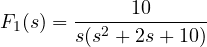
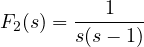
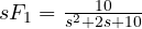
Compute, if it exists, the final value of $f$ for $F_1(s) = \dfrac{10}{s(s^2 + 2s + 10)}$ and for $F_2(s) = \dfrac{1}{s(s - 1)}$ .

Result: $f_1(\infty) = 1$ ; for $F_2$ the limit does not exist (the formula would give $-1$ , wrongly).

Solution

$sF_1 = \frac{10}{s^2 + 2s + 10}$ : poles $-1 \pm 3i$ , negative real part. The theorem applies: $\lim_{s\to 0}sF_1 = 1$ . It is the step response of a system with unit static gain.

$sF_2 = \frac{1}{s - 1}$ : pole at $+1$ , on the right. The theorem does not apply. Indeed $f_2 = e^t - 1$ (partial fractions: $\frac{1}{s - 1} - \frac{1}{s}$ ), which diverges. The formula would give $-1$ , a meaningless number.

The case where the final value does not exist — The function e to the t minus 1 diverges; the value minus 1 given by the formula has no meaning.

Exercise 8. Inverting with convolution

Find the inverse transform of $F(s) = \dfrac{1}{(s^2 + 1)^2}$ using convolution.

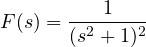
Result: $f(t) = \frac{1}{2}(\sin t - t\cos t)$ .

Solution

$F = \frac{1}{s^2 + 1}\cdot\frac{1}{s^2 + 1}$ , and each factor is the transform of $\sin t$ . So $f = \sin * \sin$ :

$f(t) = \int_0^t\sin\tau\sin(t - \tau)\,d\tau = \frac{1}{2}\int_0^t\left[\cos(2\tau - t) - \cos t\right]d\tau = \frac{1}{2}\left[\frac{\sin(2\tau - t)}{2}\right]_0^t - \frac{t\cos t}{2}$

The first term equals $\frac{1}{2}\cdot\frac{\sin t + \sin t}{2} = \frac{\sin t}{2}$ . Result: $\frac{1}{2}(\sin t - t\cos t)$ .

Meaning: it is the response of an undamped oscillator $y'' + y = \sin t$ driven at its resonant frequency. The amplitude grows linearly with time: double poles on the imaginary axis are unstable.

Resonance — The solution oscillates with an amplitude that grows linearly in time, inside the dashed lines plus and minus t over 2.

Exam level

Exercise 9. An RLC circuit switched on to a step

A series RLC circuit with $R = 2$ Ω, $L = 1$ H, $C = 0.2$ F, initially uncharged, is connected at time 0 to a 10 V source. Find the current $i(t)$ .

Result: $i(t) = 5\,e^{-t}\sin 2t$ A.

Solution

In the $s$ domain (lesson): inductor $sL$ , capacitor $\frac{1}{sC}$ , source $\frac{10}{s}$ . Mesh law:

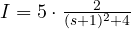
$I(s)\left(R + sL + \frac{1}{sC}\right) = \frac{10}{s} \quad\Rightarrow\quad I(s) = \frac{10}{Ls^2 + Rs + 1/C} = \frac{10}{s^2 + 2s + 5}$

Poles $-1 \pm 2i$ . $I = 5\cdot\frac{2}{(s + 1)^2 + 4}$ , so $i(t) = 5e^{-t}\sin 2t$ A.

Checks: $i(0) = 0$ (the inductor prevents jumps in current); $i(\infty) = 0$ (the charged capacitor blocks DC). The circuit is underdamped because $R \lt 2\sqrt{L/C} = 4.47$ Ω: with a larger resistance the current would not oscillate.

Current in the RLC circuit — The current starts from zero, rises to about 2.6 A, changes sign and dies out oscillating.

Exercise 10. The specifications of a second-order system

A system has transfer function $G(s) = \dfrac{4}{s^2 + 2s + 4}$ . Find $\omega_n$ , $\zeta$ , the overshoot, the peak time and the 2 % settling time of the step response.

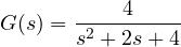
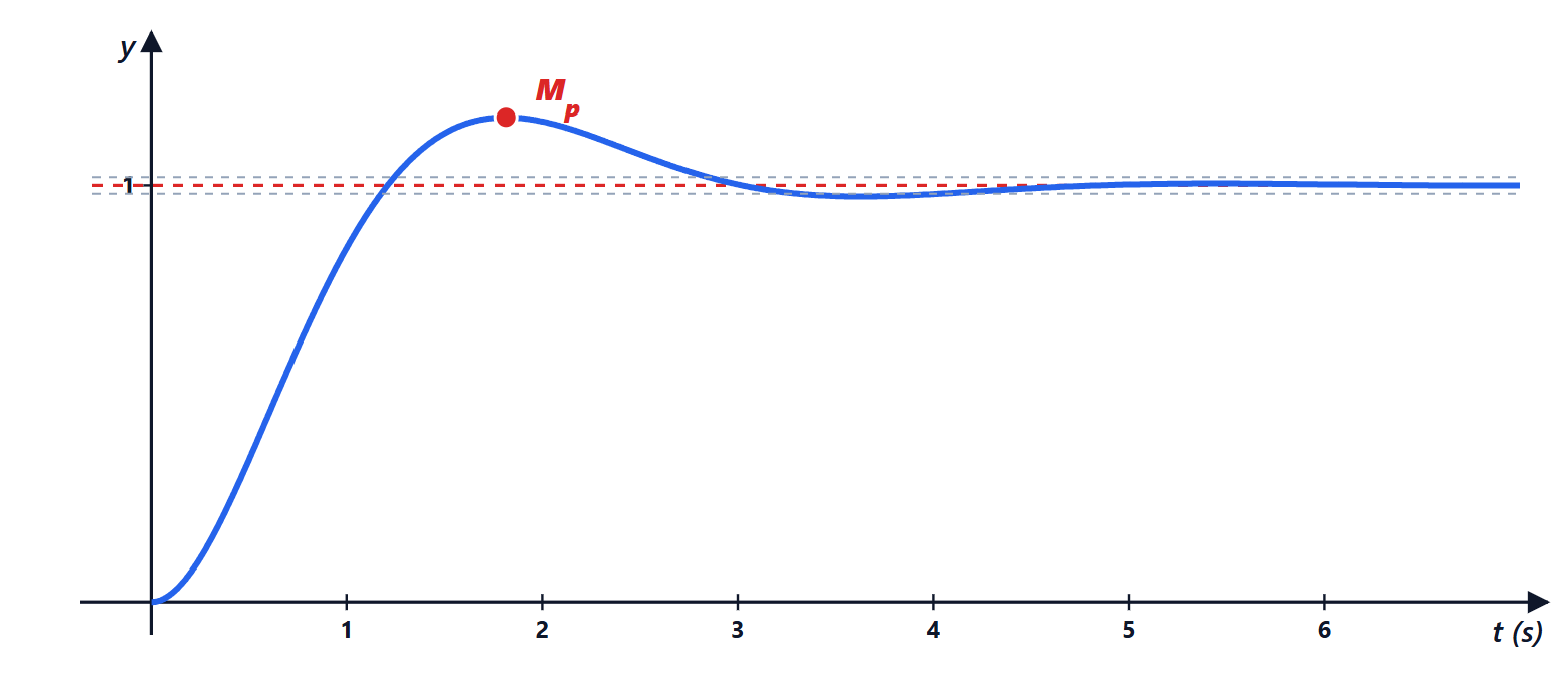
Result: $\omega_n = 2$ rad/s, $\zeta = 0.5$ ; $M_p = 16.3$ %; $t_p = 1.81$ s; $t_s \approx 4$ s.

Solution

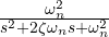
Comparison with the standard form $\frac{\omega_n^2}{s^2 + 2\zeta\omega_ns + \omega_n^2}$ : $\omega_n^2 = 4$ , $\omega_n = 2$ ; $2\zeta\omega_n = 2$ , $\zeta = 0.5$ .

$M_p = e^{-\pi\cdot 0.5/\sqrt{0.75}} = e^{-1.814} = 0.163$ . $t_p = \frac{\pi}{2\sqrt{0.75}} = 1.81$ s. $t_s \approx \frac{4}{0.5\cdot 2} = 4$ s. Static gain $G(0) = 1$ : the output goes to 1.

The formulas come from the step response $y = 1 - \frac{e^{-\zeta\omega_nt}}{\sqrt{1 - \zeta^2}}\sin(\omega_dt + \arccos\zeta)$ : the peak is where the derivative first vanishes, i.e. $\omega_dt = \pi$ .

Step response of the second-order system — The output exceeds the final value 1 by 16 per cent at the peak time, red dot, and then enters the 2 per cent band, grey lines.

Exercise 11. A periodic signal

Find the transform of the square wave with period $T = 2$ that is 1 for $0 \le t \lt 1$ and 0 for $1 \le t \lt 2$ .

Result: $F(s) = \dfrac{1}{s(1 + e^{-s})}$ .

Solution

Transform of the first period: $F_1 = \int_0^1 e^{-st}dt = \frac{1 - e^{-s}}{s}$ . With the formula for periodic signals:

$F = \frac{F_1}{1 - e^{-2s}} = \frac{1 - e^{-s}}{s(1 - e^{-s})(1 + e^{-s})} = \frac{1}{s(1 + e^{-s})}$

Poles: $s = 0$ and the zeros of $1 + e^{-s}$ , i.e. $s = i(2k + 1)\pi$ : the odd harmonics $\pi, 3\pi, 5\pi, \dots$ rad/s, exactly those of the Fourier series of the square wave (Analysis 2 lesson). The mean value $\frac{1}{2}$ corresponds to the pole at 0: $\lim_{s\to 0}sF = \frac{1}{2}$ .

Square wave with period 2 — The signal is 1 between 0 and 1, 0 between 1 and 2, and so on.

Exercise 12. An integral equation

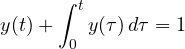
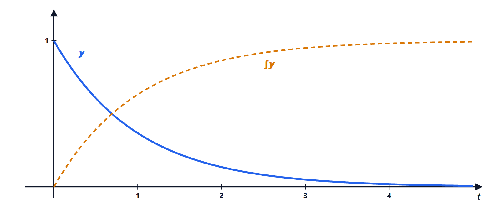
Find $y(t)$ such that $y(t) + \displaystyle\int_0^t y(\tau)\,d\tau = 1$ for $t \ge 0$ .

Result: $y(t) = e^{-t}$ .

Solution

Transforming, the integral becomes a division by $s$ : $Y + \frac{Y}{s} = \frac{1}{s}$ . So $Y\cdot\frac{s + 1}{s} = \frac{1}{s}$ and $Y = \frac{1}{s + 1}$ , i.e. $y = e^{-t}$ .

Check: $\int_0^t e^{-\tau}d\tau = 1 - e^{-t}$ , and $e^{-t} + 1 - e^{-t} = 1$ .

It is the law of an RC circuit seen from the current: the voltage across the resistor plus that across the capacitor (integral of the current) equals the source. Equations of this kind (Volterra equations) appear in models with memory, and Laplace turns them into algebra.

Solution of the integral equation — The solution e to the minus t, in blue, and its integral, dashed, always add up to 1.

0 Comments

Oldest

Newest Most Voted

Cookie	Duration	Description
cookielawinfo-checkbox-analytics	11 months	This cookie is set by GDPR Cookie Consent plugin. The cookie is used to store the user consent for the cookies in the category "Analytics".
cookielawinfo-checkbox-functional	11 months	The cookie is set by GDPR cookie consent to record the user consent for the cookies in the category "Functional".
cookielawinfo-checkbox-necessary	11 months	This cookie is set by GDPR Cookie Consent plugin. The cookies is used to store the user consent for the cookies in the category "Necessary".
cookielawinfo-checkbox-others	11 months	This cookie is set by GDPR Cookie Consent plugin. The cookie is used to store the user consent for the cookies in the category "Other.
cookielawinfo-checkbox-performance	11 months	This cookie is set by GDPR Cookie Consent plugin. The cookie is used to store the user consent for the cookies in the category "Performance".
viewed_cookie_policy	11 months	The cookie is set by the GDPR Cookie Consent plugin and is used to store whether or not user has consented to the use of cookies. It does not store any personal data.

Basic level

Exercise 1. A power times an exponential

Exercise 2. The square of sine

Exercise 3. A double pole at the origin

Exercise 4. Complex conjugate poles

Intermediate level

Exercise 5. A differential equation with initial conditions

Exercise 6. A piecewise signal

Exercise 7. The final value theorem, used well and used badly

Exercise 8. Inverting with convolution

Exam level

Exercise 9. An RLC circuit switched on to a step

Exercise 10. The specifications of a second-order system

Exercise 11. A periodic signal

Exercise 12. An integral equation

Related articles

Solved limit exercises, from basic to exam level

Solved exercises on current, DC circuits and the RC circuit

Solved curve-sketching exercises, with graphs

Laplace transform in depth: convergence, properties, final value and inverse transform in every case

Integrals in depth: fundamental theorem, integration methods proved and tables

Solved Fourier transform exercises, with graphs