Solved Fourier transform exercises, with graphs
Twelve exercises with solutions: exponentials, delayed pulses, convolution, modulation, duality, Parseval, RC filter, in-band energy, aliasing, uncertainty principle.
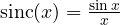
Exercises on the Fourier transform of the kind set in Mathematical Methods for Engineering and Signal Theory courses, in three levels: basic, with transforms from the definition; intermediate, with properties, convolution, duality and Parseval; exam, with filters, energy, sampling and the uncertainty principle. The result is given straight away; the full solution, with the graph, opens with a click. Convention:  ;
 .
Basic level
Exercise 1. The two-sided exponential
Compute the transform of 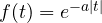 , with
 .
Result:  .
Solution
Split the integral over the two half-lines:

The integrals converge because . The transform is real and even, like the signal (a real even signal has a real even spectrum). The shape  is called a Lorentzian: it is the spectrum of the noise coming out of an RC filter.

Exercise 2. The one-sided exponential: magnitude and phase
Compute the transform of  and write its magnitude and phase. What are they at
 ?
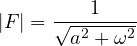
Result:  ;
 ,
 ; at :
 and
 .
Solution
 .
Multiplying by the conjugate: 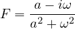 , so and
 .
At the magnitude is  of its value at 0 (i.e.
 dB) and the phase is . This is the cut-off frequency of the RC filter, with
 : the impulse response of the filter is exactly
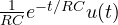 .

Exercise 3. A delayed pulse
Compute the transform of the pulse that is 1 for  and 0 elsewhere. What changes compared with the pulse centred at the origin?
Result:  ; the magnitude is the same, the phase becomes linear.
Solution
The pulse has duration  and is centred at
 : it is
 . The centred pulse has transform
 (lesson), and by the delay property it is multiplied by
 :

The magnitude  does not change: the amplitude spectrum does not say when the signal occurs. The phase changes, adding
 : a straight line with slope equal to minus the delay. This is why a filter that must not distort a signal must have linear phase (all frequencies delayed by the same time).

Exercise 4. The triangle as a convolution
Show that the convolution of  with itself is the triangle
 (base from
 to 1, height 1) and derive the transform of the triangle.
Result:  .
Solution
 is the length of the overlap between the interval
 and the same interval shifted by
 . It is 1 for
 and decreases linearly to 0 for
 :
 , the triangle.
By the convolution theorem the transform is the product:  .
Computing it directly from the definition would take two integrations by parts: convolution is a powerful shortcut.

Intermediate level
Exercise 5. Amplitude modulation
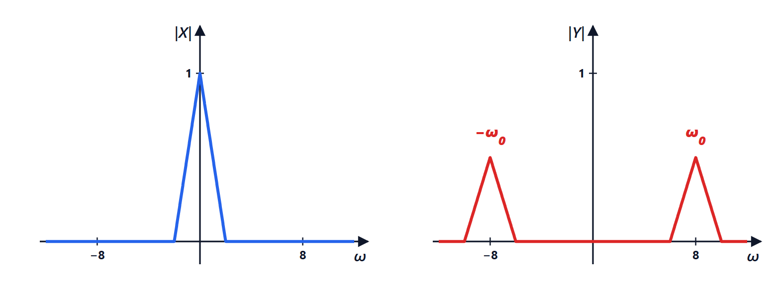
A signal  has a triangular spectrum, zero for
 . It is transmitted as
 . Sketch the spectrum of
 and explain how
 is recovered.
Result:  : two halved copies centred at
 .
Solution
 , and by the modulation property each exponential shifts the spectrum: .
The copies occupy the bands  and do not overlap because
 . To recover (demodulation) multiply again by
 : this gives
 , and a low-pass filter removes the term at angular frequency 16. This is the scheme of every AM radio and, with small variations, of digital transmission.
Exercise 6. Duality
Knowing that  , compute the transform of
 without integrating.
Result:  .
Solution
Duality: if  , then
 . With
 ,
 :

Computing it directly would require the residue theorem (lesson). Check:  , the area of the signal.
Note that the signal is smooth (infinitely differentiable) and the spectrum decays exponentially; the spectrum has a peak at 0 and the signal decays only as  . Smoothness on one side, decay on the other.

Exercise 7. An integral with Parseval
Use Parseval’s theorem to compute 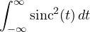 .
Result:  .
Solution
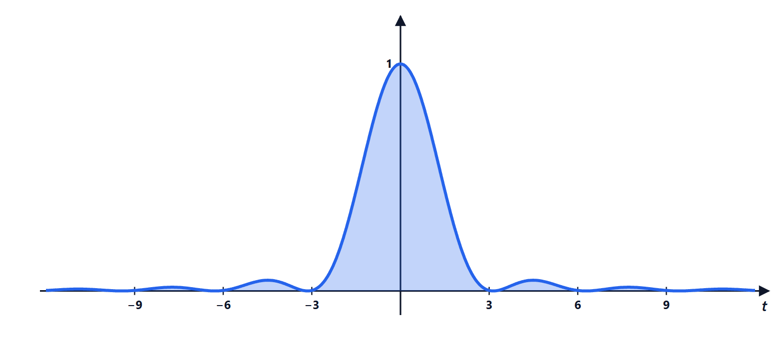
The pulse  (1 for
 ) has transform
 . Parseval:

The left-hand side is 2 (the duration). So  .
An integral that is hard in time becomes trivial in frequency. With the same idea, using the transform itself instead of Parseval (area = value of the transform at 0), one also finds  .
Exercise 8. Differentiation in frequency
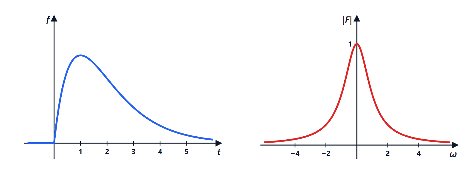
Compute the transform of  using the property
 .
Result:  .
Solution
With 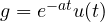 ,
 and
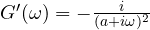 . So
 .
Magnitude: , which decays as  : the signal is continuous at 0 (it is 0 on both sides), but its derivative jumps from 0 to 1. This is exactly the decay rule of the in-depth study.
Exam level
Exercise 9. A pulse through an RC filter
A rectangular pulse of amplitude 1 and duration enters an RC filter with  . Compute the output in time with convolution and explain the result in frequency.
Result:  for
 ,
 for
 ;
 .
Solution
Impulse response  . The output is
 .
For :  . For :
 . At the end of the pulse
 .
In frequency.  . The filter attenuates the components beyond
 rad/s: they are the ones that make up the steep edges, which indeed become exponential. The main lobe of the pulse spectrum (up to rad/s) passes almost entirely, and the output gets close to level 1. With
 much larger than
 the output would stay small: the filter would “not have time” to follow the pulse.

Exercise 10. How much energy is in the band
For the signal , what fraction of the energy lies in the band  ?
Result: 50 %.
Solution
Total energy in time:  .
In frequency, 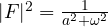 , and the energy in the band is

Fraction:  %. To contain 90 % one would need
 : the slow tails of the Lorentzian make the bandwidth of a signal with a jump wide.

Exercise 11. Aliasing
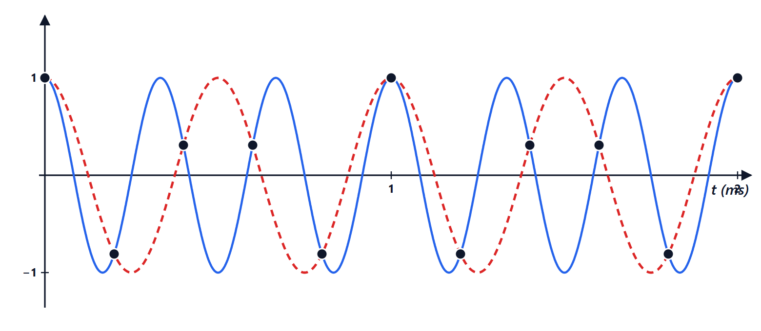
A signal  is sampled at 5 kHz. What frequency does the processor “see”? And if it were sampled at 8 kHz?
Result: 2 kHz with 5 kHz sampling; 3 kHz (correct) with 8 kHz.
Solution
With  kHz the Nyquist limit is 2.5 kHz, and 3 kHz exceeds it. The samples are
 . Since
 , they are identical to those of a cosine at
 Hz.
In general the apparent frequency is the distance from the nearest multiple of  :
 kHz. The processor has no way of telling them apart: the information is lost at the moment of sampling.
At 8 kHz the limit is 4 kHz and the 3 kHz signal is represented correctly.
Exercise 12. The uncertainty principle for the Gaussian
For  , compute the duration
 and the bandwidth
 defined as in the in-depth study, and check that the product is
 .
Result:  ,
 , product .
Solution
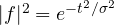 is a Gaussian with variance
 (compare with
 :
 ). The weighted mean of
 is the variance:
 .
In frequency  , a Gaussian with variance
 :
 .
Product:  , the minimum possible. No other signal is as concentrated in time and frequency: this is why Gaussian pulses are used in radar and communications (GMSK modulation in GSM, Bluetooth).