The Dirac delta, distributions and the impulse response
The delta as a limit and as a distribution, the derivative of the step, impulse response and convolution, transforms of constants, sines and the step, the Dirac comb and sampling.
Engineers used the Dirac delta “function” long before mathematicians could say what it was: an infinitely short and infinitely tall pulse with area 1. It is not a function in the usual sense but a distribution. With this concept the transforms of a sine, a constant and the step make sense, and the impulse response becomes the tool for describing any linear system.
The idea: a pulse of unit area
Consider the rectangle  of width
 and height
 , centred at the origin. Its area is always 1. Letting tend to zero gives a “pulse” concentrated at
 .
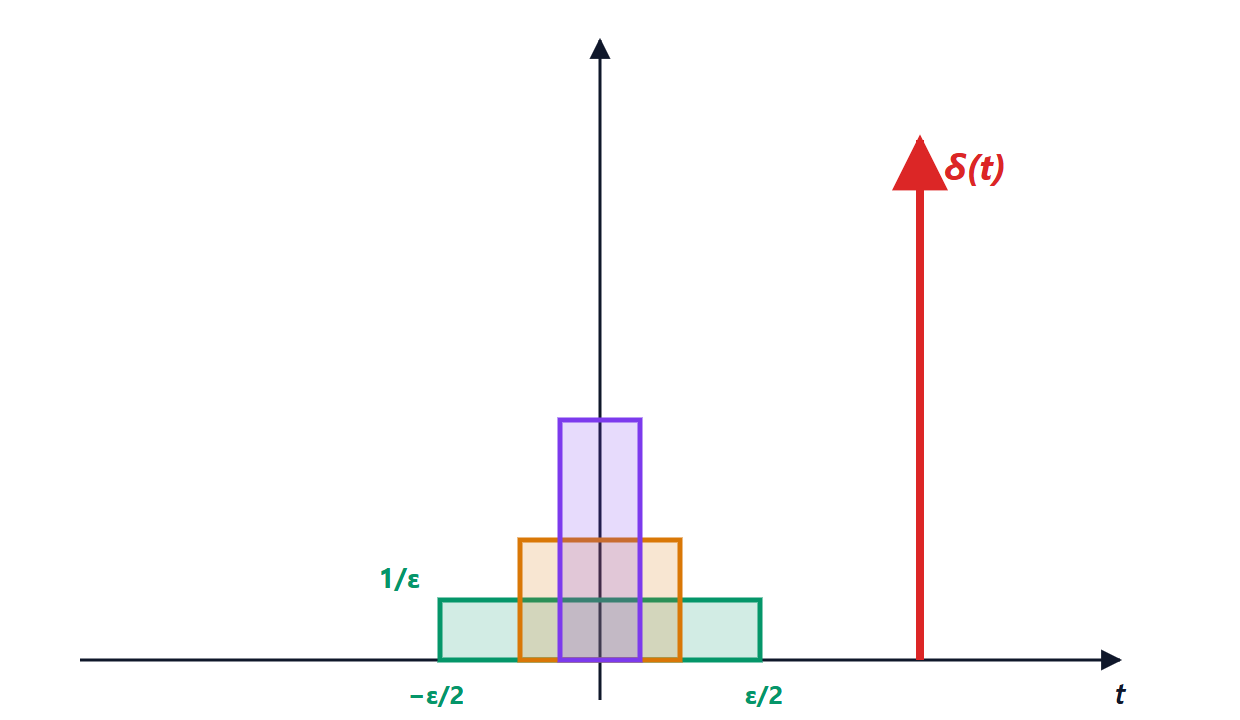
As a function the limit makes no sense (it would be 0 everywhere except at one point where it is infinite, and its integral would be zero). But the effect of the rectangles on a continuous function  has a precise limit:

because the average of over a shrinking interval tends to its value at the centre (mean value theorem for integrals).
The definition
The Dirac delta is defined by its action on smooth functions:

The delta “samples” the function at the point  . More generally, a distribution is a linear and continuous way of assigning a number to each test function (infinitely differentiable and zero outside a bounded interval). Ordinary functions are distributions, through
 ; the delta is a distribution that does not come from any function.
Useful properties.
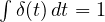 ;
 ;
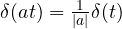 ;
 : the delta is the identity element of convolution.
The derivative of the step
The unit step  is 0 for
 and 1 for
 : it describes a switch closing. As a function it is not differentiable at 0. As a distribution it is: integrating by parts, for every test function

so

The derivative of a jump is an impulse with area equal to the jump. It is the right language for circuits: the current that charges an ideal capacitor when a switch closes onto a constant voltage, 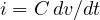 , is exactly an impulse, and in a real circuit it is “spread out” by the resistance of the wires.
The impulse response
A linear time-invariant system is completely described by its impulse response  , the output when the input is
 . Indeed any input can be written as a “sum” of impulses:
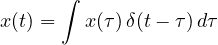
By linearity and time invariance, each impulse  produces
 , so

It is the convolution of the lesson on the Fourier transform, now proved. A system is causal (it does not respond before being excited) if  for , and stable (bounded input, bounded output) if
 is finite.
Example. An RC low-pass circuit has  : after the kick, the capacitor voltage jumps up and then decays exponentially. In acoustics the impulse response of a hall is measured with a starter pistol or a bursting balloon, and then used to simulate that hall’s echo on any recording.
Fourier transforms that did not exist before
With the delta, signals that are not integrable can be transformed.
| Signal | Fourier transform |
|---|---|
|  |
|  |
 |  |
 |  |
| 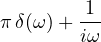 |
The first row reads: an impulse contains every frequency with the same amplitude. That is why lightning interferes with every radio station, and why the impulse response holds all the information about the system: its transform is exactly the frequency response  .
The fourth row says that a pure sinusoid has a spectrum made of two lines, at  : what you see on a spectrum analyser when a sinusoidal signal is applied.
The Dirac comb and sampling
The comb  , a train of impulses with period
 , has as its transform another comb, with period
 in frequency. Sampling a signal means multiplying it by the comb; in the frequency domain the multiplication becomes a convolution, which copies the spectrum around every multiple of the sampling frequency. It is the compact proof of the sampling theorem seen in the lesson on the Fourier transform.