Policy gradient and PPO: REINFORCE, baseline, actor-critic, GAE and clipped objective

DQN learns values and derives the policy from them. One can also do the opposite: parameterise the policy directly with a neural network and move its weights in the direction that increases the average return. These are policy gradient methods. They work with continuous actions (torques, steering, acceleration), learn stochastic policies and are the basis of PPO (Proximal Policy Optimization, Schulman et al., 2017), the most used algorithm today: from walking robots to language models trained with human feedback. This lesson proves the policy gradient theorem, derives REINFORCE, the baseline and actor-critic, explains the generalised advantage (GAE) and the “clipped” objective of PPO, and applies it to CartPole.

The policy gradient theorem

The objective is the average return , where is a trajectory and its return.

Theorem. , with the return from onwards.

Proof. The probability of a trajectory is . The log-derivative trick is used, :

In the logarithm the product becomes a sum, and the terms and do not depend on : they vanish when differentiating. What remains is . Finally the rewards received before do not depend on , and their contribution has zero mean (by the same argument as the baseline below): can be replaced by . ∎

The result is remarkable: to improve the policy the model of the environment is not needed, it is enough to be able to differentiate one’s own policy. The interpretation is intuitive: increase the probability of actions followed by a high return, decrease that of actions followed by a low return. Estimating the average with the played trajectories gives the REINFORCE algorithm (Williams, 1992).

The baseline and actor-critic

REINFORCE is correct but very slow: has an enormous variance. A baseline can be subtracted without changing the mean.

Lemma. .

Proof. . ∎

The natural choice is : instead of the advantage is used, which says how much better than expected the action went. is learned with a second network, the critic, while the policy is the actor: this is the actor-critic scheme, the “evaluate and improve” version of policy iteration.

Generalised advantage (GAE). As between Monte Carlo and TD, the advantage can be estimated with the TD error (low variance, biased) or with the whole return (unbiased, high variance). GAE (Schulman, 2016) takes an exponential average:

with one gets the TD error, with the Monte Carlo return minus ; usually . The recursive form is computed backwards in one line of code.

PPO: big steps but not too big

A gradient step that is too long can change the policy so much as to ruin it, and the data collected with the old policy are no longer valid. PPO uses the probability ratio 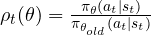between the new policy and the one that collected the data, and maximises the clipped objective:

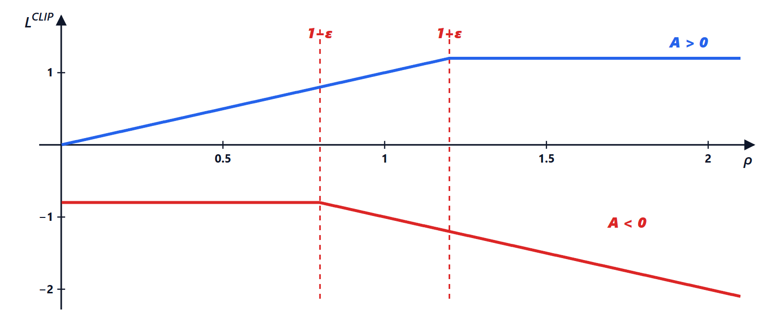
with . If an action was good () its probability is increased, but beyond 20 % more the objective becomes flat and the gradient vanishes; if it was bad () its probability is reduced, but not below 20 % less. The minimum guarantees that clipping acts only when it would improve the objective, never when it worsens it: it is a pessimistic bound on the gain. In this way several steps (epochs) can be taken safely on the same data. The critic error and a small entropy bonus, which keeps exploration alive, are added to the objective.

PPO on CartPole

The code collects 128 steps from 8 environments in parallel (1024 transitions), computes GAE, performs 4 update epochs with the clipped objective and repeats 100 times. The environments are vectorised with PufferLib, presented in the lesson on libraries; with Gymnasium (gymnasium.vector.SyncVectorEnv) the code would be almost identical.

import numpy as np
import torch, torch.nn as nn
import gymnasium
import pufferlib.emulation, pufferlib.vector

N_ENV, T, UPDATES = 8, 128, 100                  # 8 environments, 128 steps each per update
GAMMA, LAM, CLIP, LR, EPOCHS = 0.99, 0.95, 0.2, 1e-3, 4
torch.manual_seed(0)

def make(buf=None, seed=0):
    return pufferlib.emulation.GymnasiumPufferEnv(env=gymnasium.make("CartPole-v1"), buf=buf, seed=seed)
envs = pufferlib.vector.make(make, num_envs=N_ENV, backend=pufferlib.vector.Serial)
obs, _ = envs.reset(seed=0)

actor = nn.Sequential(nn.Linear(4, 64), nn.Tanh(), nn.Linear(64, 64), nn.Tanh(), nn.Linear(64, 2))
critic = nn.Sequential(nn.Linear(4, 64), nn.Tanh(), nn.Linear(64, 1))
params = list(actor.parameters()) + list(critic.parameters())
opt = torch.optim.Adam(params, lr=LR)

for k in range(UPDATES):
    for g in opt.param_groups:
        g["lr"] = LR * (1 - k / UPDATES)                # learning rate decreasing linearly to zero
    O, A, LP, R, D, V = [], [], [], [], [], []
    for t in range(T):                                  # data collection with the current policy
        o = torch.tensor(obs, dtype=torch.float32)      # copy: PufferLib reuses the same buffer
        with torch.no_grad():
            dist = torch.distributions.Categorical(logits=actor(o))
            a = dist.sample()
            O.append(o); A.append(a); LP.append(dist.log_prob(a)); V.append(critic(o).squeeze(-1))
        obs, r, term, trunc, _ = envs.step(a.numpy())
        R.append(torch.tensor(r, dtype=torch.float32))
        D.append(torch.tensor(np.logical_or(term, trunc), dtype=torch.float32))
    with torch.no_grad():
        v_end = critic(torch.tensor(obs, dtype=torch.float32)).squeeze(-1)
    adv, last = torch.zeros(T, N_ENV), torch.zeros(N_ENV)
    for t in reversed(range(T)):                        # GAE, computed backwards
        v_next = v_end if t == T - 1 else V[t + 1]
        delta = R[t] + GAMMA * v_next * (1 - D[t]) - V[t]
        last = delta + GAMMA * LAM * (1 - D[t]) * last
        adv[t] = last
    returns = (adv + torch.stack(V)).reshape(-1)
    O, A, LP = torch.stack(O).reshape(-1, 4), torch.stack(A).reshape(-1), torch.stack(LP).reshape(-1)
    adv = adv.reshape(-1)
    adv = (adv - adv.mean()) / (adv.std() + 1e-8)
    for _ in range(EPOCHS):                             # clipped PPO objective
        dist = torch.distributions.Categorical(logits=actor(O))
        ratio = torch.exp(dist.log_prob(A) - LP)
        loss_pi = -torch.min(ratio * adv, torch.clamp(ratio, 1 - CLIP, 1 + CLIP) * adv).mean()
        loss_v = ((critic(O).squeeze(-1) - returns) ** 2).mean()
        loss = loss_pi + 0.5 * loss_v - 0.01 * dist.entropy().mean()
        opt.zero_grad(); loss.backward()
        nn.utils.clip_grad_norm_(params, 0.5)
        opt.step()
envs.close()

env, scores = gymnasium.make("CartPole-v1"), []
for e in range(10):                                     # evaluation with the most likely action
    o, _ = env.reset(seed=100 + e)
    tot, done = 0.0, False
    while not done:
        with torch.no_grad():
            o, r, te, tr, _ = env.step(int(actor(torch.tensor(o, dtype=torch.float32)).argmax()))
        tot += r; done = te or tr
    scores.append(tot)
print("evaluation over 10 episodes:", np.mean(scores))
torch.save(actor.state_dict(), "expert.pt")             # will serve as the expert to imitate

In less than 10 seconds on a processor (about 100,000 steps) the average return of the last 20 episodes during training goes from 162 after 20 updates to 245, 201, 401 and 407 (during training actions are still random), and the evaluation with the most likely action gives 500 on all 10 episodes. Two tricks were decisive in the trials: the learning rate decreasing to zero and the gradient norm limit (0.5); without them, the policy reached 400 and then got worse. This is typical of RL: results change a lot with hyperparameters and with the random seed, and several seeds are always used to compare two methods. A simplification: the code also treats the time limit (500 steps) as terminal, which strictly would require continuing to bootstrap; for CartPole the effect is small.

Why PPO is everywhere

It is simple (a few lines beyond actor-critic), more robust to hyperparameters than many competitors, works with discrete and continuous actions and parallelises well over thousands of simulated environments. It is the algorithm with which OpenAI trained the robotic hand that solved the Rubik’s cube and the Dota 2 bots, and the one used in 2022 for InstructGPT, the language model that made training with human feedback (RLHF) famous, as shown in the lesson on applications.