The Deep Q-Network (DQN): replay memory, target network and double DQN on CartPole

A table works as long as states are few. CartPole has four continuous variables, an Atari video game has 210×160 pixel images: states are infinite or astronomically many. In 2015 DeepMind showed that a convolutional neural network, trained with Q-learning and two tricks, learns to play 49 Atari games starting only from pixels, surpassing human level in many. This is the Deep Q-Network (DQN). This lesson explains why Q-learning with a neural network is unstable, how the replay memory and the target network stabilise it, why the maximum overestimates values (and the remedy, double DQN), and applies it to CartPole with code that reaches the maximum score.

From tabular Q-learning to the network

The table is replaced by a function with parameters (the weights of a network): the state as input, one value per action as output. The Q-learning update becomes a gradient descent step on the loss

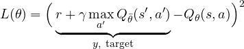
where the target is treated as a constant (no derivative is taken with respect to it). It looks simple, but put together naively it often diverges.

Why it diverges: the deadly triad

Sutton and Barto call the deadly triad the combination of three ingredients that, together, can make learning diverge even in simple problems:

• function approximation: changing to correct also changes the values of similar states one did not want to touch;
• bootstrapping: the target contains the estimate itself , so an error propagates and feeds itself;
• off-policy: the greedy policy is learned from data collected with another policy (the exploring one).

Deep Q-learning has all three. To these a statistical problem is added: consecutive steps of an episode are strongly correlated (the state at step is almost equal to that at step ), while gradient descent assumes independent examples.

The two DQN tricks

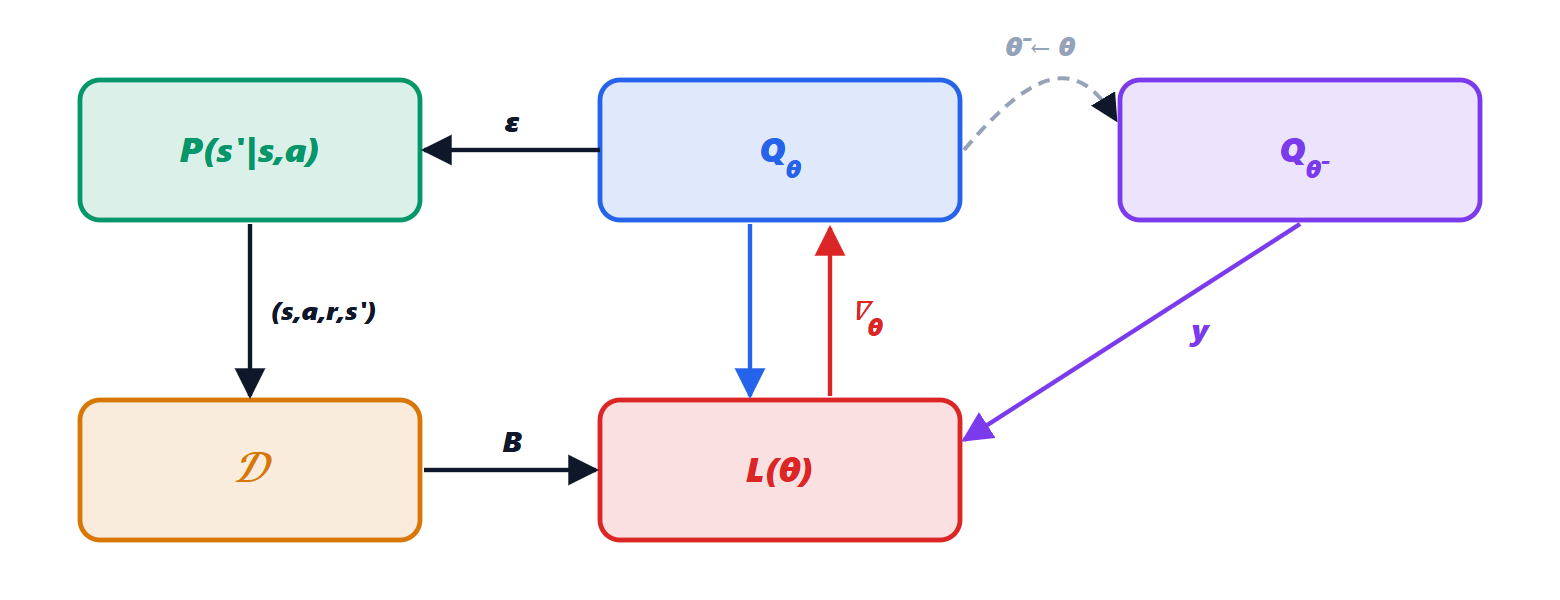
Replay memory. Every transition is stored in a buffer of a few tens of thousands of elements; at each training step a mini-batch is drawn at random. This breaks correlations, reuses every experience many times (which is legitimate because Q-learning is off-policy) and averages over many different situations.

Target network. The target is computed with a copy of the weights, , updated only every few hundred or thousand steps (). Between two copies the problem becomes a supervised regression with fixed targets, and the network does not “chase its own tail”.

Overestimation of the maximum and double DQN

Theorem. If the estimates are unbiased but noisy, , then the maximum is overestimated: .

Proof. For every , ; taking the average, , and this holds for every , hence also for the one maximising . ∎

Noise gets “selected”: the action that looks best is often the one estimated too high. The overestimation accumulates through bootstrapping. Double DQN (van Hasselt, 2016) separates choice from evaluation: the online network chooses the action, the target network evaluates it,

The errors of the two networks are largely independent, and the overestimation is greatly reduced.

True end and time limit. If the episode ends because the pole fell, there is no further reward and the target is just . If instead it ends because time ran out (500 steps in CartPole), the state is not terminal: the target must still include . Confusing the two cases is one of the most common mistakes; Gymnasium distinguishes them with the two values terminated and truncated.

The code on CartPole

import random, collections
import numpy as np
import torch, torch.nn as nn
import gymnasium

torch.manual_seed(0); random.seed(0); np.random.seed(0)
env = gymnasium.make("CartPole-v1")

def network():
    return nn.Sequential(nn.Linear(4, 128), nn.ReLU(), nn.Linear(128, 128), nn.ReLU(), nn.Linear(128, 2))
q, q_target = network(), network()
q_target.load_state_dict(q.state_dict())
opt = torch.optim.Adam(q.parameters(), lr=2.5e-4)
memory = collections.deque(maxlen=10000)                      # replay memory
STEPS, BATCH, GAMMA, COPY, EVERY, START = 200000, 128, 0.99, 500, 10, 10000

o, _ = env.reset(seed=0)
env.action_space.seed(0)
for t in range(STEPS):
    eps = max(0.05, 1 - 0.95 * t / 100000)                   # decreasing exploration
    if random.random() < eps:
        a = env.action_space.sample()
    else:
        with torch.no_grad():
            a = int(q(torch.tensor(o, dtype=torch.float32)).argmax())
    o2, r, terminated, truncated, _ = env.step(a)
    memory.append((o, a, r, o2, float(terminated)))           # only a true end zeroes the future
    o = o2
    if terminated or truncated:
        o, _ = env.reset()
    if t >= START and t % EVERY == 0:
        b = random.sample(memory, BATCH)
        O, A, R, O2, D = (torch.tensor(np.array(x), dtype=torch.float32) for x in zip(*b))
        with torch.no_grad():                                 # double DQN
            a2 = q(O2).argmax(1, keepdim=True)
            y = R + GAMMA * (1 - D) * q_target(O2).gather(1, a2).squeeze(1)
        estimate = q(O).gather(1, A.long().unsqueeze(1)).squeeze(1)
        loss = nn.functional.mse_loss(estimate, y)
        opt.zero_grad(); loss.backward(); opt.step()
    if t % COPY == 0:
        q_target.load_state_dict(q.state_dict())            # target network update

# greedy evaluation over 20 episodes
scores = []
for e in range(20):
    o, _ = env.reset(seed=1000 + e)
    tot, done = 0.0, False
    while not done:
        with torch.no_grad():
            o, r, te, tr, _ = env.step(int(q(torch.tensor(o, dtype=torch.float32)).argmax()))
        tot += r; done = te or tr
    scores.append(tot)
print("evaluation:", np.mean(scores))

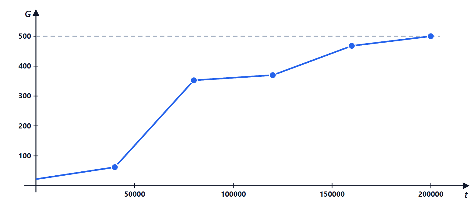
The hyperparameters are those of the CleanRL teaching library. During training the average return goes from 62 (after 40,000 steps) to 353, 370, 468 and 500; the final greedy evaluation is 500 over 20 episodes, the maximum possible. On an ordinary processor it takes less than a minute.

Beyond DQN

DQN works with few discrete actions (it must compute the maximum over all of them). For continuous actions, such as a robot’s torques or a car’s steering, actor-critic methods (DDPG, TD3, SAC) are used, which also learn a policy, together with the policy gradient methods of the next lesson. The DQN variants for games (Rainbow) add prioritised replay, “dueling” networks, multi-step returns and return distributions; the principle remains the one described here.