Simulation for RL: MuJoCo, Isaac, sim-to-real, domain randomisation and Gaussian splatting

An RL agent needs millions of trials, and no real robot or car can fall a million times. This is why almost all applied reinforcement learning happens in simulation: the agent is trained in a virtual world and then transferred to the real one. This lesson presents the most used physics simulators, the problem of the gap between simulation and reality (sim-to-real gap) and the techniques to bridge it, and finally Gaussian splatting, a 2023 technique that reconstructs photographed real scenes and renders them in real time, increasingly used to build photorealistic simulators for robots and autonomous vehicles.

Physics simulators

• MuJoCo (Multi-Joint dynamics with Contact): a physics engine for articulated bodies with contacts, born for robotics and become the RL standard for continuous control (Gymnasium’s locomotion environments use it). Acquired by DeepMind in 2021 and made open source in 2022. MJX is its JAX version, running on the GPU.
• Isaac Sim and Isaac Lab (NVIDIA): physics and sensor simulation on the GPU, with thousands of simulated robots in parallel in the same process. Training locomotion for a quadruped robot thus takes minutes instead of days.
• Brax (Google): differentiable physics written in JAX, very fast on the GPU.
• CARLA: an open-source simulator for autonomous driving, based on a video game engine, with cities, traffic, pedestrians, weather and sensors (cameras, LiDAR, radar).

The common principle is the one seen with PufferLib: speed comes from running many environments together in compiled code or on the GPU, without returning to Python at every step.

The gap between simulation and reality

A simulator is never perfect: masses, friction, motor delays, sensor noise and surface appearance are always slightly different. A policy optimised too well for the simulator exploits its defects (for example a friction slightly too high) and fails in the real world. The main techniques:

• system identification: measuring the parameters of the real robot (masses, inertias, friction, latencies) and putting them in the simulator, as is done for a classic controller;
• domain randomisation: at each episode the parameters are drawn at random (mass ±20 %, friction between 0.5 and 1.2, sensor delay, colours and lighting of images). The policy learns to work on a whole family of worlds, and the real world becomes “one of many”. OpenAI used it in 2019 to have a robotic hand trained only in simulation solve the Rubik’s cube, automatically widening the ranges as the agent improved;
• actuator networks: a model of the motors’ behaviour is learned from real data and inserted into the simulation (this was decisive in making ETH Zurich’s ANYmal quadruped robot run in 2019);
• online adaptation: the policy also receives an estimate of the parameters (or the recent history of states and actions) as input and adapts by itself.

Gaussian splatting

For tasks with cameras (autonomous driving, robots that see) the simulated images must also resemble the real ones. Modelling every building and every tree by hand takes a long time and the result never looks real. The alternative is to reconstruct the scene from real photos or video. In 2020 NeRFs (neural radiance fields) showed that a neural network can learn a scene from a few dozen photos, but rendering took seconds per image. In 2023 Kerbl, Kopanas, Leimkühler and Drettakis presented 3D Gaussian splatting: similar quality, real-time rendering.

The representation. The scene is a set of millions of three-dimensional Gaussians, small ellipsoidal “clouds”. Each has:

• a position (the centre);
• a covariance giving its shape and orientation, written as with a rotation and a diagonal matrix of the three scales: in this way it always stays symmetric and positive definite during optimisation;
• an opacity ;
• a colour that changes with the viewing direction (described with spherical harmonics, for reflections).

Rendering. Each Gaussian is projected onto the image: with the view transformation and the Jacobian of the perspective projection, its footprint on the screen is a two-dimensional Gaussian with covariance . The Gaussians are sorted by depth and composited front to back, like overlapping semi-transparent sheets:

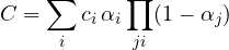
where is the opacity of Gaussian at the pixel (the opacity times the value of the Gaussian at that point) and the product is the light that reaches there without being absorbed by the previous ones. Everything is computed in parallel on the GPU, in tiles of pixels, at more than 100 images per second.

Training. One starts from the 3D points obtained from the photos with photogrammetry (structure from motion) and optimises all parameters with gradient descent, comparing rendered images with the real photos. The compositing formula is differentiable, so the pixel error can be “traced back” to the position, shape, colour and opacity of every Gaussian. During optimisation Gaussians that are too large are split, those in under-described areas are duplicated, transparent ones are removed.

Why it matters for RL. With a few tens of minutes of video of a junction, a warehouse or a stretch of road one obtains a navigable, photorealistic scene, from which images can be rendered from new viewpoints: those a vehicle making a manoeuvre different from the recorded one would see. Policies using cameras can thus be trained and tested in closed loop in the reconstructed “real” world, and the dangerous situations missing from recordings can be generated. It is one of the most active routes to reducing the gap between simulation and reality in perception.

A two-dimensional example

The following code applies the same ideas to a flat image: 150 two-dimensional Gaussians with position, two scales, rotation, colour and opacity, composited with the front-to-back formula and optimised with Adam to reproduce a 64×64 pixel image.

import torch

torch.manual_seed(0)
H = W = 64
yy, xx = torch.meshgrid(torch.linspace(0, 1, H), torch.linspace(0, 1, W), indexing="ij")
img = torch.zeros(H, W, 3) + torch.tensor([0.10, 0.15, 0.35])            # image to reconstruct
img[((xx - 0.35) ** 2 + (yy - 0.40) ** 2) < 0.18 ** 2] = torch.tensor([0.95, 0.55, 0.10])
u, v = (xx - 0.68) * 0.8 + (yy - 0.62) * 0.6, -(xx - 0.68) * 0.6 + (yy - 0.62) * 0.8
img[(u.abs() < 0.18) & (v.abs() < 0.08)] = torch.tensor([0.20, 0.75, 0.35])
img[(yy - 0.85).abs() < 0.03] = torch.tensor([0.95, 0.95, 0.95])

N = 150
pos = torch.rand(N, 2, requires_grad=True)                 # centres
log_s = torch.full((N, 2), -3.0, requires_grad=True)       # scales (as logarithms: always positive)
rot = torch.zeros(N, requires_grad=True)                   # rotations
col = torch.rand(N, 3, requires_grad=True)                 # colours (before the sigmoid)
op = torch.zeros(N, requires_grad=True)                    # opacities (before the sigmoid)

def render():
    c, s, S = torch.cos(rot), torch.sin(rot), torch.exp(log_s)
    dx, dy = xx[None] - pos[:, 0, None, None], yy[None] - pos[:, 1, None, None]
    u = (c[:, None, None] * dx + s[:, None, None] * dy) / S[:, 0, None, None]     # coordinates in the
    v = (-s[:, None, None] * dx + c[:, None, None] * dy) / S[:, 1, None, None]    # Gaussian's axes
    alpha = torch.sigmoid(op)[:, None, None] * torch.exp(-0.5 * (u ** 2 + v ** 2))
    light = torch.cumprod(torch.cat([torch.ones(1, H, W), 1 - alpha[:-1]], 0), 0) # product of (1 - alpha_j)
    return ((alpha * light)[..., None] * torch.sigmoid(col)[:, None, None, :]).sum(0)

psnr = lambda a, b: float(10 * torch.log10(1 / ((a - b) ** 2).mean()))
opt = torch.optim.Adam([pos, log_s, rot, col, op], lr=0.02)
print(f"initial: PSNR {psnr(render().detach(), img):.1f} dB")
for it in range(1, 1501):
    loss = ((render() - img) ** 2).mean()                   # pixel error
    opt.zero_grad(); loss.backward(); opt.step()             # the gradient reaches every Gaussian
    if it in (100, 500, 1500):
        print(f"iteration {it}: PSNR {psnr(render().detach(), img):.1f} dB")

The peak signal-to-noise ratio (PSNR, higher is better) rises from 10.8 dB at the start to 23.3 dB after 100 iterations, 29.5 after 500 and 31.0 after 1500, in about 40 seconds on a processor. In the three-dimensional case the perspective projection, depth sorting and the number of Gaussians (millions) change, but the principle is this one: a set of simple primitives, a differentiable rendering formula, gradient descent.