Monte Carlo and temporal differences: SARSA and Q-learning on the cliff example
Learning values from experience: Monte Carlo, TD(0), convergence conditions, on-policy SARSA and off-policy Q-learning, the cliff example with safe and optimal path, verified code.
https://www.electronics-engineering.com/en/temporal-differences-sarsa-q-learning-cliff/
The Bellman equations require knowing the transition probabilities  and the rewards
 . They are almost never known: a robot has no formula for how it will slip on the floor, a game does not say in advance the opponent’s moves. One can however try and observe what happens. This lesson presents the methods that learn values from experience: Monte Carlo, which waits for the end of the episode, and temporal differences (TD), which update at every step. From these come SARSA and Q-learning, which we compare on the classic cliff example, with code and results.
Monte Carlo: the average of returns
Value is an average:  . The most direct way to estimate it is to play many episodes following
 , compute the return
 every time
 is visited and average. In incremental form, after each observed return:

with  the learning rate. With
 (n number of visits) it is exactly the arithmetic mean. Monte Carlo makes no assumptions about the environment, but it must wait for the end of the episode and its estimates have high variance: sums many random rewards.
Temporal differences
Sutton’s idea (1988) is to replace the true return, known only at the end, with an estimate built from the Bellman equation:  . The TD(0) update is

Learning happens at every step, even in tasks without an end. The estimate uses another estimate (it is said to bootstrap): it has less variance than Monte Carlo, because it depends on a single random reward, but it is biased as long as  is wrong. The bias-variance trade-off between Monte Carlo and TD is tuned with
 -step returns and the parameter
 (TD(), and in its modern version the GAE used by PPO).
Convergence. With a table, if every state is visited infinitely often and the step sizes satisfy the Robbins-Monro conditions,  and
 (for example
 ), TD(0) converges to
 with probability 1. The idea of the proof: on average the update applies the Bellman operator, which is a contraction; the first condition allows reaching anywhere, the second switches off the noise.
From value to action: SARSA and Q-learning
To choose actions without a model  is needed, not
 : with one would need to know where each action leads. Exploring with an ε-greedy policy (best action according to
 with probability
 , random with probability
 ), is updated after each transition
 :


The only difference is the target. SARSA uses the action  the agent will actually take (exploration included): it learns the value of the policy it is following, and is called on-policy. Q-learning uses the maximum, i.e. the action the optimal policy would take: it learns
 whatever the way it explores, and is called off-policy (Watkins, 1989). Being off-policy is precisely what allows reusing old experience or experience collected by others, and it is the basis of DQN.
The cliff example
A 4×12 grid: the start is at the bottom left, the exit at the bottom right, and the bottom cells between them are a cliff: falling in gives  and sends back to the start. Each step costs
 . The shortest path runs along the edge of the cliff (13 steps); a safer one goes higher.
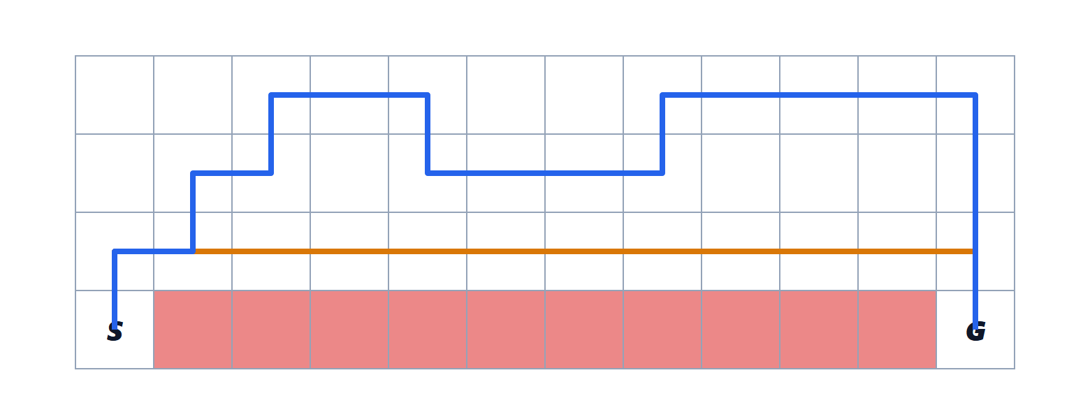
With  ,
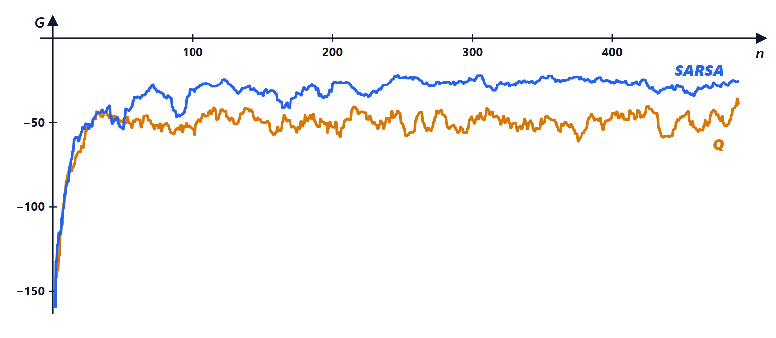
 and 500 episodes (average over 20 random seeds):
| learned path | average return in the last 100 episodes | |
|---|---|---|
| SARSA | safe, 19 steps | −28.1 |
| Q-learning | optimal, 13 steps | −48.0 |
Q-learning finds the best path, but earns less while learning: walking on the edge, the 10 % random move makes it fall often. SARSA knows it will explore and prefers to stay away from the edge. It is a lesson that applies to real systems: a robot learning on a real plant must take its own exploration into account, and on-policy or “cautious” algorithms are often preferable; in simulation, where falling costs nothing, one can use Q-learning and then switch off exploration.
The code
import numpy as np

ROWS, COLS = 4, 12
START, EXIT = (3, 0), (3, 11)
MOVES = [(-1, 0), (1, 0), (0, -1), (0, 1)]

def step(pos, a):
    r = min(max(pos[0] + MOVES[a][0], 0), ROWS - 1)
    c = min(max(pos[1] + MOVES[a][1], 0), COLS - 1)
    if r == 3 and 1 <= c <= 10:            # cliff: -100 and back to the start
        return START, -100.0, False
    return (r, c), -1.0, (r, c) == EXIT

def learn(method, episodes=500, alpha=0.5, eps=0.1, seed=0):
    rng = np.random.default_rng(seed)
    Q = np.zeros((ROWS, COLS, 4))
    def choose(p):                          # epsilon-greedy (tiny noise to break ties)
        return rng.integers(4) if rng.random() < eps else int(np.argmax(Q[p] + 1e-9 * rng.random(4)))
    returns = []
    for _ in range(episodes):
        p, tot = START, 0.0
        a = choose(p)
        for _ in range(1000):
            p2, r, done = step(p, a)
            tot += r
            a2 = choose(p2)
            if method == "sarsa":
                target = r if done else r + Q[p2][a2]               # action actually chosen
            else:
                target = r if done else r + np.max(Q[p2])           # best action
            Q[p][a] += alpha * (target - Q[p][a])
            p, a = p2, a2
            if done:
                break
        returns.append(tot)
    return np.array(returns), Q

for method in ("sarsa", "qlearning"):
    curves = np.array([learn(method, seed=s)[0] for s in range(20)])
    _, Q = learn(method, seed=0)
    p, length, done = START, 0, False
    while not done and length < 50:         # final greedy path
        p, _, done = step(p, int(np.argmax(Q[p])))
        length += 1
    print(f"{method:9s}: last 100 episodes {curves[:, -100:].mean():6.1f}, path of {length} steps")
Running it prints  and 19 steps for SARSA,
 and 13 steps for Q-learning. A table with one cell per state-action pair works as long as states number a few thousand; for CartPole (continuous states) or a video game (states made of pixels) an approximation is needed: the table becomes a neural network, the DQN of the next lesson.


Sono l'autore di questa pagina su «Monte Carlo e differenze temporali: SARSA e Q-learning sull’esempio della scogliera». Se qualcosa non è chiaro, se vi serve un esempio in più o volete approfondire un punto, scrivetelo qui sotto nei commenti: rispondo personalmente. Se la pagina vi è stata utile, lasciate un voto con le stelle in cima all'articolo.I am the author of this page on “Monte Carlo and temporal differences: SARSA and Q-learning on the cliff example”. If something is unclear, if you need another example or want to go deeper into a point, write it in the comments below: I answer personally. If the page was useful, leave a star rating at the top of the article.