The sampling theorem and aliasing
Ideal sampling, the Nyquist-Shannon theorem with proof and sinc reconstruction, aliasing with examples, the anti-aliasing filter, oversampling and undersampling.
To process a signal with a computer it must be turned into a sequence of numbers, by taking its value at regular intervals: sampling. The natural question is whether something is lost this way. The sampling theorem gives a surprising answer: if the signal is band-limited and is sampled fast enough, nothing is lost, and the original signal can be reconstructed exactly. In this lesson we prove it and see what happens when the conditions are not met.
Ideal sampling
Sampling  with period
 (sampling frequency
 ) gives the values
 . To study them with the Fourier transform they are represented as a train of weighted impulses:

The sampling theorem
Theorem (Nyquist-Shannon). If  for
 and
 , the signal is determined by its samples and is reconstructed by

Proof. The impulse train is periodic, with Fourier series  . Multiplying by
 shifts the spectrum by
 , so
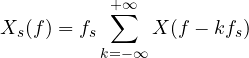
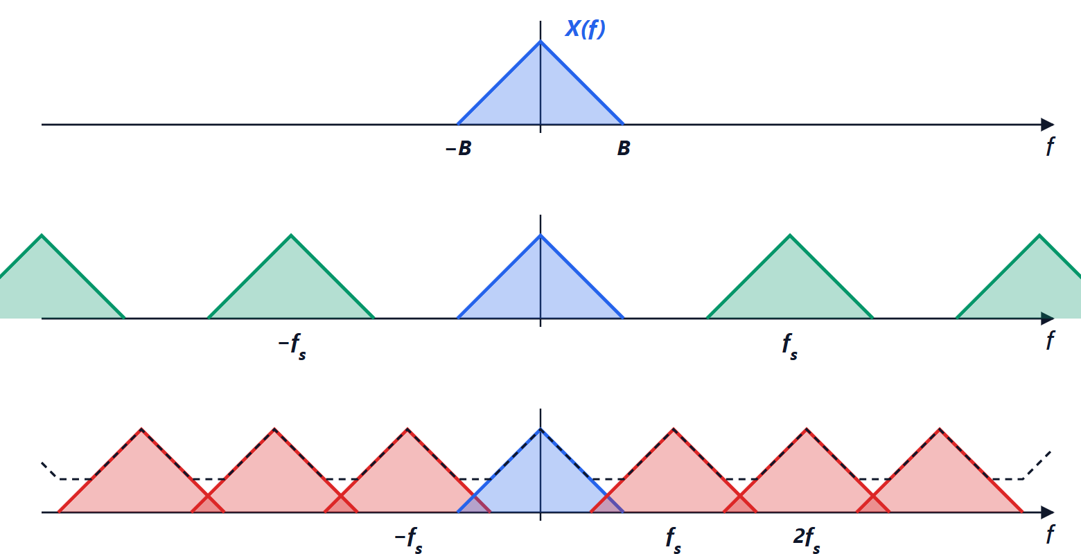
The spectrum of the sampled signal is the sum of replicas of the original spectrum, centred at all multiples of  . If , the replicas, each
 wide, do not overlap: an ideal low-pass filter with cut-off at
 and gain isolates the central replica, that is
 . In time, filtering means convolving with the filter’s impulse response, which is
 ; convolving each impulse
 with the sinc gives the formula. ∎
The frequency is called the Nyquist rate. Each sample “carries” a sinc, and the sum of the sincs passes exactly through all the samples and interpolates between them.
Aliasing
If  , the replicas overlap and the components above fold back into the low band, mixing with the real ones: this is aliasing, and after sampling there is no way to separate them. A component at frequency
 appears at the nearest frequency
 , for the appropriate integer
 .
Example. Sampling a 30 kHz tone at 44.1 kHz gives the same samples as a tone at  kHz: an audible whistle that was not in the original.
It is the same phenomenon that makes carriage wheels in films seem to turn backwards: the camera samples at 24 frames per second and a rotation that is too fast is “seen” as a slow one.
Sampling in practice
- Anti-aliasing filter. Before the converter, an analogue low-pass filter removes everything above , including unwanted noise: once sampled, it can no longer be removed.
- Margin. A real filter has a transition band, so sampling is done somewhat above . Audio CDs sample at 44.1 kHz for a signal up to 20 kHz: the filter has between 20 and 22.05 kHz to go from transparent to blocking.
- Oversampling. Sampling much faster than necessary lets the analogue filter be simple, and the rest of the filtering is done digitally. Almost all modern audio converters work this way.
- Reconstruction. A digital-to-analogue converter holds each sample constant until the next (zero-order hold): the output is a staircase, which a final low-pass filter smooths.
Sampling narrowband signals
The theorem requires where  is the highest frequency. For a bandpass signal, for example a radio channel between 100 and 101 MHz, a sampling rate tied to the width of the band (1 MHz) is actually enough, as long as the replicas fall in the right places: this is undersampling, used in software-defined radios. Alternatively the signal is first shifted around zero with a mixer and then sampled.