Digital control: sampling, period choice and velocity-form PID
The zero-order hold as a half-period delay with proof, choosing the sampling period, anti-aliasing, the position PID, the velocity form proved, anti-windup and bumpless transfer.
Today almost no controller is analogue: the PID is a program running in a PLC, in a distributed control system (DCS) or in a microcontroller, and it reads the measurement at regular instants. The step from continuous to discrete has precise consequences: an extra delay in the loop, a choice to make about the sampling period, and some forms of the algorithm that are more convenient than others. In this lesson we prove that sample-and-hold is equivalent to a delay of half a period, look at how to choose the period, how the PID is discretised and why the velocity form solves two practical problems by itself.
Sample and hold
The digital controller reads the measurement every  seconds, computes the command and holds it constant until the next computation: this is the zero-order hold (ZOH), implemented by the digital-to-analogue converter or simply by the output not changing.
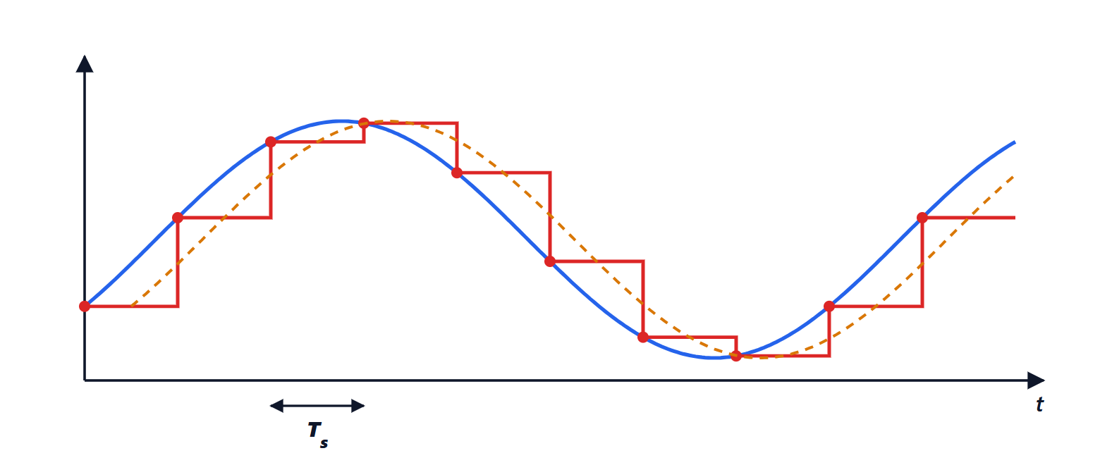
Theorem. At frequencies low compared with the sampling frequency, the zero-order hold is equivalent to a delay of  .
Proof. The transfer function of the hold, normalised to unit static gain, is
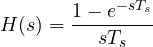
because its impulse response is a rectangle of duration and height  . Setting
 , factor out
 :

For small  ,
 , and what remains is
 : a pure delay of half a period. ∎
The computation time adds to the hold delay, if the command is applied at the next sample. All this is extra dead time in the loop, and the lesson on processes with dead time says how much it costs.
Choosing the sampling period
The added delay must be small compared with the loop dynamics. The practical rules are:
- between one tenth and one twentieth of the desired closed-loop time constant;
- no more than a quarter of the process dead time, if the latter dominates;
- for industrial processes, typical values are 0.1-1 s for flows and pressures, 1-10 s for temperatures and levels, minutes for composition analysis.
Sampling too fast is not free: the derivative computed as a difference between close samples amplifies noise and converter resolution, and the computations load the CPU. An anti-aliasing filter is always needed before the converter (Signal Theory lesson on sampling): a 50 Hz disturbance sampled at 1 s would appear as a slow, non-existent oscillation, and the controller would try to correct it.
Discretising the PID
The integral is approximated by a sum and the derivative by a difference. With the backward (Euler) method, at instant  :

This is the position form: it computes the value of the command directly. The Tustin method (trapezoidal rule) is more accurate for the same period and preserves the stability of continuous systems; for periods short compared with the dynamics, as used in practice, the differences are small. The derivative must be filtered anyway, and computed on the measurement rather than on the error.
The velocity form
Theorem. The discrete PID can be written in incremental (or velocity) form:

Proof. Write the position form at instant and at instant  and subtract. The proportional part gives
 . In the integral sum all the terms up to cancel and
 remains. The derivative gives
 , which is the term written. ∎
The two forms are equivalent as long as the output meets no limits, but the velocity form has two important practical advantages:
- no integrator winding up: the state is the command itself,
 . If the valve is fully open and the command is limited to 100 %, the next step starts from 100 % and not from an internal value that kept growing. Anti-windup is automatic: just saturate
 ;
- bumpless transfer from manual to automatic: in manual the operator sets
 ; when switching to automatic the algorithm starts from the last value and changes it only by increments, without jumps.
That is why the velocity form has for decades been the one used in industrial controllers and in the PID blocks of PLCs.
Other implementation details
- Set-point weighting: the proportional term is computed on
 with
 , to reduce the kick on the valve at set-point changes without changing the disturbance response.
- Resolution and dead band: with a 12-bit converter the step is 0.025 % of the span; a small dead band on the error prevents the valve from moving all the time because of noise, wearing out its packing.
- Rate limit: a limit on the rate of change of the command protects actuators and process from abrupt changes.
- Fault handling: if the measurement is out of range or the sensor has failed, the controller goes to manual holding the last valid command, or drives the output to a safe position.