Multivariable systems: relative gain array and pairing
Process with two inputs and two outputs, Bristol's relative gain with proof, rows and columns summing to one, the pairing rule, a distillation column example, decoupling and model predictive control.
In a real plant the control loops are not independent: opening a valve to correct a temperature also changes a pressure, which another controller corrects, in turn disturbing the temperature. When the interactions are strong, tuning each loop well on its own is not enough. In this lesson we look at the model of a process with several inputs and outputs, Bristol’s relative gain array (RGA) with the proof of its properties, the rule for pairing inputs and outputs, decoupling and predictive control.
The process with two inputs and two outputs
The simplest case has two manipulated variables  and two controlled ones
 , each affected by both inputs:

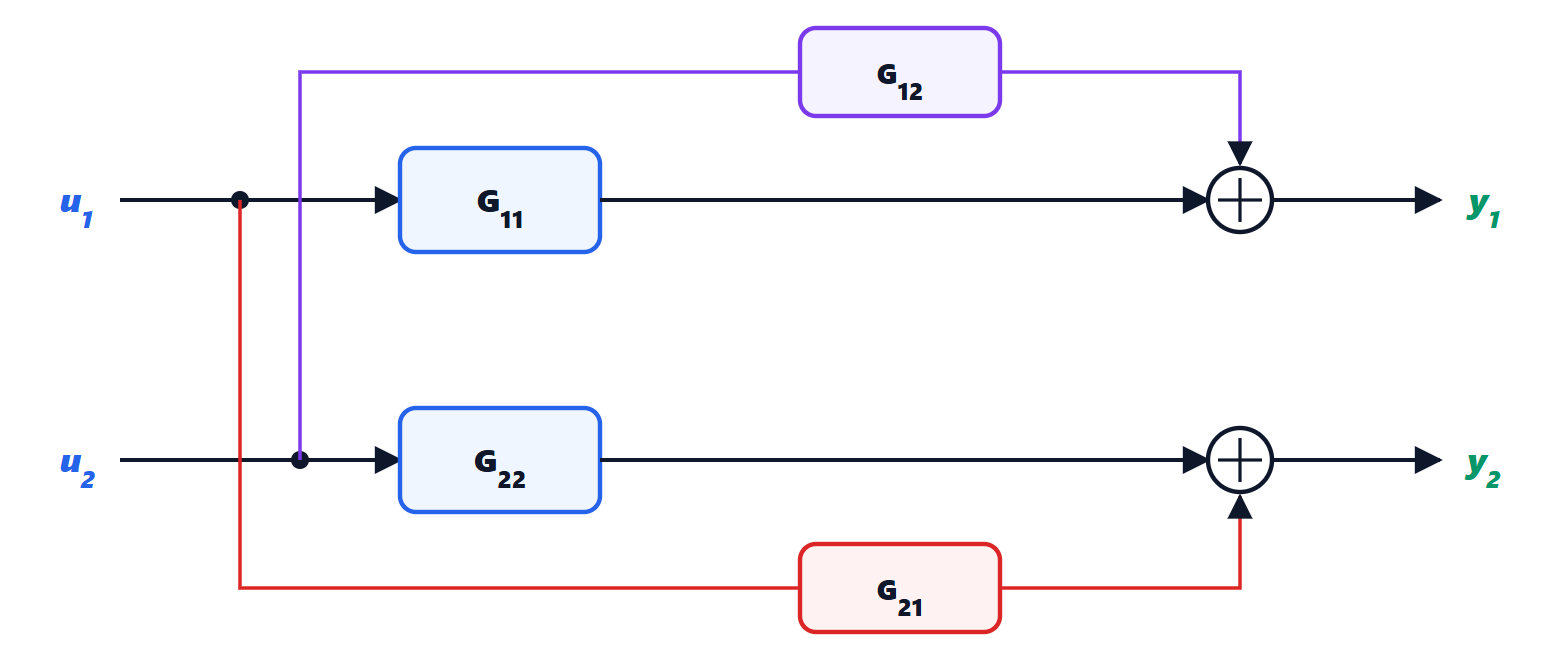
A classic example is a mixing tank fed with hot and cold water: the outputs are the total flow and the temperature, and each of the two valves changes both. Another is the distillation column, where the reflux and the reboiler heat affect both purities, top and bottom.
If two separate loops are closed,  on
 and
 on
 , controller 1 no longer sees the gain
 : it sees a gain modified by the action of controller 2, which reacts to each of its moves. A measure of how much this interaction matters is needed.
The relative gain
We work with the static gains  .
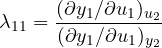
Definition. The relative gain between and is the ratio between the gain from to with the other loop open ( constant) and the same gain with the other loop closed and perfect ( constant):
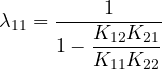
Theorem. For a 2×2 process
Proof. With constant the gain is simply  . With constant, the second equation imposes
 , so a change of changes by
 . Substituting into the first equation:

The ratio of the two gains is  , and dividing numerator and denominator by gives the formula. ∎
The other elements are computed in the same way, and are collected in the relative gain array (RGA).
Theorem. In every row and every column of the RGA the elements sum to 1. For a 2×2 process the matrix is therefore determined by  :
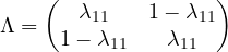
Proof (2×2 case). Let  , so
 . For
 , between and , the same reasoning (now adapts to keep constant:
 ) gives

and  . By symmetry the same holds for the second row and for the columns. ∎
How to read the RGA
 : the other loop does not change the gain seen by the first. No interaction, the loops are tuned separately.
 : closing the other loop increases the gain seen (the other controller “helps”). Moderate interaction if close to 1.
 : closing the other loop reduces the gain. Large values, 5, 10 or more, indicate strong interaction and a difficult process.
 : closing the other loop changes the sign of the gain. A controller tuned with the other loop open becomes positive feedback when the other closes: instability.
Bristol’s pairing rule: pair each output with the input whose relative gain is positive and closest to 1, and never pair on a negative relative gain.
Example. A classic distillation column model, much studied in the literature, has static gains
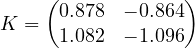
Here  and
 . The diagonal pairing is the right one (the other would have
 ), but the interaction is very strong: the two loops fight each other, and a small model error changes the behaviour a lot. Such a process is called ill-conditioned: the two outputs almost always move together, and it is hard to change only one of them.
Decoupling and predictive control
When the interaction is strong a decoupler  can be inserted between the controllers and the process so that
 is diagonal: in the static case
 , so each controller moves a combination of valves that changes only one output. On ill-conditioned processes, however, exact decoupling is fragile, for the same reason: it requires inverting an almost singular matrix.
In refineries and large chemical plants the most widespread solution today is model predictive control (MPC). A computer uses a multivariable model of the process to predict the outputs over the next minutes or hours and, at every sampling period, solves an optimisation problem: it finds the sequence of valve moves that brings the outputs to their set points while respecting all the constraints (maximum openings, temperature limits, safety pressures). It applies only the first move and repeats the calculation at the next step with the new measurements. MPC handles interactions, delays and constraints naturally; it usually does not drive the valves directly, but provides the set points to the basic PIDs, which remain the fast layer of the plant.