Processes with dead time and the Smith predictor
The bandwidth limit imposed by dead time with proof, the Smith predictor with proof, the effect of model errors and disturbances, Padé approximation, the half rule.
Dead time is the main enemy of process control. A conveyor belt, a long pipe, an analyser that takes minutes to give the composition: in all these cases the controller acts “blind” for a certain time, and if it is too aggressive it keeps correcting an error it has already corrected. In this lesson we prove the speed limit that delay imposes on any loop, look at the Smith predictor with the proof of how it works, its limits, and the approximations of the delay used in calculations.
Why delay is so difficult
A pure delay  has magnitude 1 at all frequencies and phase
 radians, which grows without bound with frequency. All the other elements of a process have bounded phase lags: a pole at most 90°. The delay instead eats phase margin at every frequency, and sooner or later uses it up.
Theorem. For a loop with delay  whose loop gain, without the delay, behaves like an integrator around the crossover frequency
 , the phase margin is
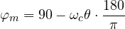
and to have at least 30° of margin one needs  , i.e. roughly
 .
Proof. With  the magnitude is 1 at
 , and the phase at that point is
 (in radians
 ). The phase margin is the distance from
 :
 in degrees. Requiring
 gives
 rad. ∎
An integrator around crossover is the ideal shape of a well-designed loop, and any other shape uses even more phase. The conclusion therefore holds in general: the closed-loop bandwidth cannot exceed about  , and the closed-loop time constant cannot go much below . This is the deep reason for the choice
 in the lesson on tuning. The first remedy, when possible, is therefore physical: bring the sensor closer to the point of action, reduce dead volumes, use a faster analyser.
The Smith predictor
In 1957 Otto Smith proposed an elegant idea: if the delay cannot be removed from the process, it can be removed from the loop, using a model. The controller receives as feedback not the real measurement, but a prediction of what the output would be if there were no delay, corrected with the difference between the measurement and the model.
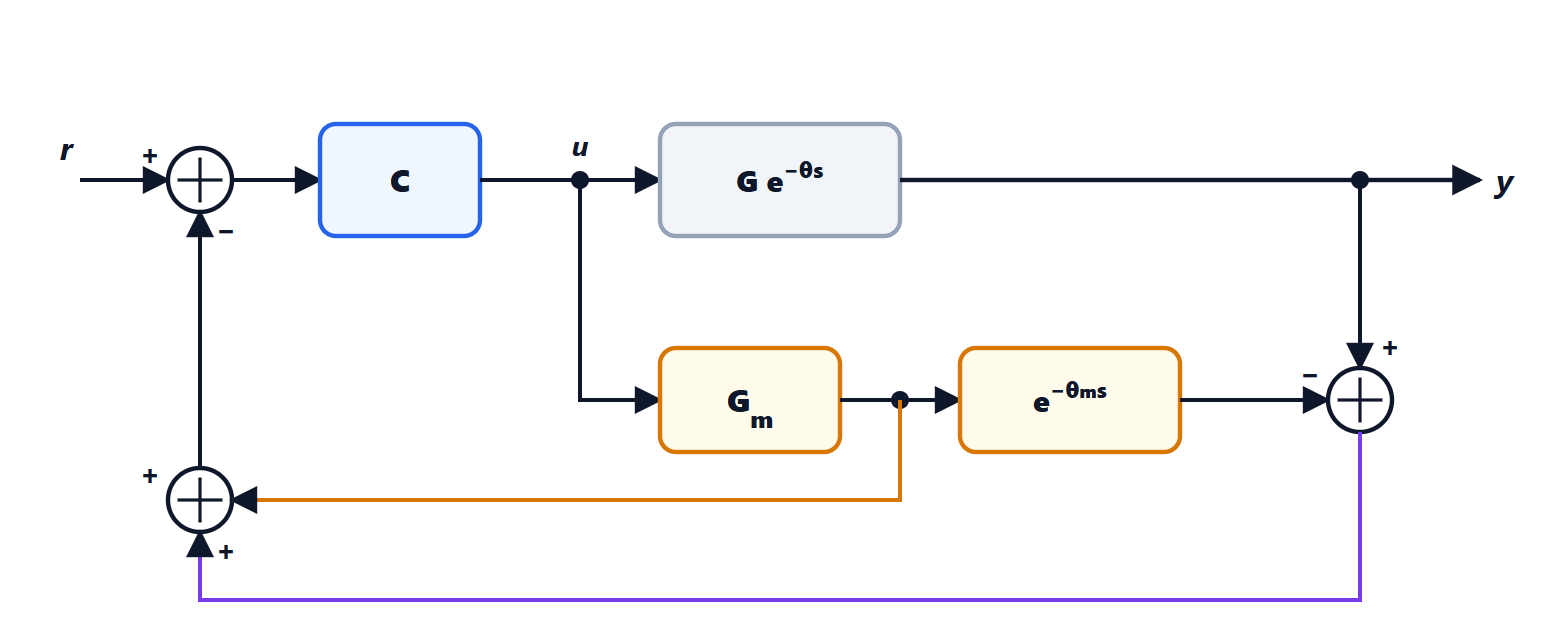
Theorem. If the model is exact ( ,
 ), with the Smith predictor
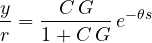
i.e. the delay leaves the characteristic equation, and the controller  is designed for the process without delay.
Proof. The feedback signal is

With 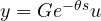 and an exact model, the term in brackets is zero, and
 : the feedback is the process output without delay. Then
 , whence
 , and

The characteristic equation is  , with no delay. ∎
The set-point response is the one that would be obtained without delay, simply shifted by : one cannot do better, because the information takes to cross the process anyway.
The limits of the predictor
- Model errors. The correction term
 is no longer zero if the model is wrong, and the delay re-enters the loop. An error in the dead time is particularly harmful: with an aggressive controller, getting wrong by 20-30 % can make the loop unstable. So the controller must be tuned cautiously, and the predictor is used where the delay is well known and constant, as in transport at fixed speed.
- Disturbances. The predictor improves the set-point response, but a disturbance entering the process is still seen only after , and its correction reaches the process after another . For disturbances the advantage over a well-tuned PI is often modest.
- Integrating processes. The basic structure does not work for unstable or integrating processes: a small difference between process and model produces an error that grows without bound. Modified versions exist for these cases.
The Smith predictor is used in paper mills and rolling mills (the thickness gauge is downstream of the machine), in furnaces and, today, in control over communication networks, where the delay is that of the network.
Approximating the delay
For calculations, simulations and design with tools that only handle rational functions, the delay is approximated:
- to first order with the Taylor series,
 , as in the direct synthesis of the lesson on tuning;
- with the first-order Padé approximation:
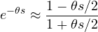
which has magnitude exactly 1 at all frequencies, like the true delay, and correct phase up to about  . It introduces, however, a zero with positive real part: the step response starts in the wrong direction instead of staying still.
Finally, when estimating a model, a set of small time constants in cascade behaves, seen from a distance, like a delay: by Skogestad’s “half rule”, the largest of the neglected constants is split in half between the main time constant and the delay, and the others are added to the delay.