Industrial process models and identification with a step test
Process variable, manipulated variable and set point, models from mass balances, dead time, the first-order-plus-dead-time model, the two-point method proved, a heat exchanger example, integrating processes.
Process control is automatic control applied to industrial plants: refineries, power stations, chemical and food plants, water networks, paper mills. The quantities to be regulated are temperatures, pressures, flows, levels and compositions, the processes are slow and often poorly known, and the most widely used controller is still the PID. In this lesson we look at the vocabulary of the field, the simple models that are enough to tune controllers and how to obtain them from a single step test, with the proof of the two-point method.
The vocabulary of plants
In every control loop there are three quantities:
- the process variable (PV): the one that is measured and is to be kept at the desired value, for instance the outlet temperature of a heat exchanger;
- the set point (SP);
- the manipulated variable (MV), on which the controller acts: almost always the opening of a valve, or the speed of a pump.
Compared with the control systems seen in the Automatic Control course, the main objective is different: the set point changes rarely, while disturbances (changes in load, in cooling water temperature, in the composition of raw materials) arrive continuously. It is a regulation problem more than a tracking one. In plant drawings (P&IDs) every loop has a tag: TIC is a temperature indicating controller, FIC a flow controller, LIC a level controller, PIC a pressure controller.
Models from physics
Many processes are described by a mass or energy balance.
A tank. With cross-section  , inlet flow
 and outlet flow
 , the mass balance gives
 . If the outlet flows freely through a hydraulic resistance,
 , and a first-order system with time constant
 is obtained. If instead the outlet is set by a pump, does not depend on
 and the level is the integral of the difference between the flows: an integrating process, which does not settle by itself.
A pipe. If the measurement is taken at a distance  from where the action takes place, and the fluid flows at speed
 , every change reaches the sensor after a dead time
 . Pure delay is one of the most typical, and most troublesome, features of industrial processes.
The first-order-plus-dead-time model
Most stable processes, even high-order ones, are well approximated by the three-parameter model
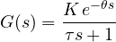
with gain  , time constant
 and dead time
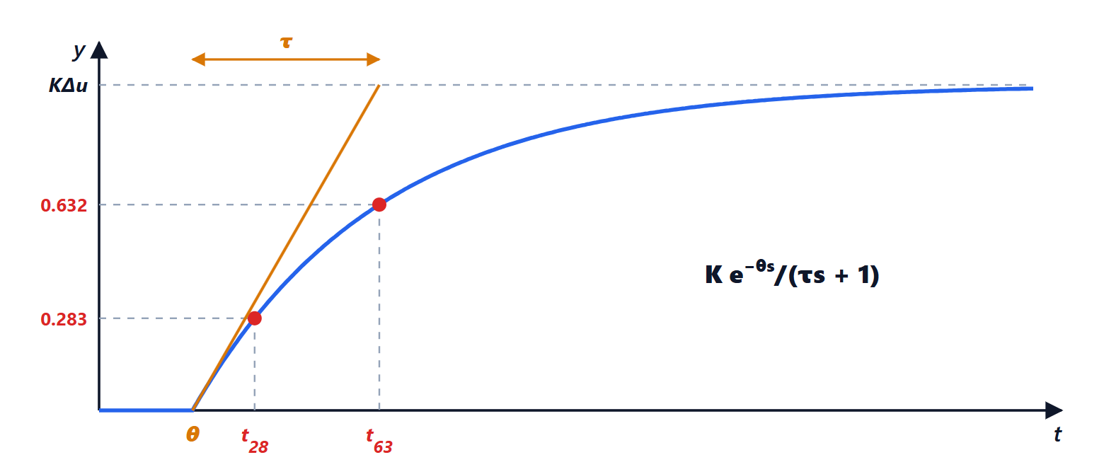
 . It is the FOPDT (first order plus dead time) model. Its response to a step of amplitude
 is zero until , then

The ratio  says how difficult the process is: below 0.1 it is easy and can be controlled aggressively; above 1 the delay dominates, and no controller can respond faster than the delay itself (lesson on processes with dead time).
Identification with a step test
With the controller in manual, a step is applied to the manipulated variable, for instance from 40 to 50 % opening, and the response is recorded. The gain is the ratio between the final change of the output and that of the input:  . For the time constant and the delay two particular instants are used.
Theorem (two-point method). Let  and
 be the instants at which the response reaches 28.3 % and 63.2 % of the final change. Then

Proof. From the response, the fraction reached at time  is
 . Since
 ,
 ; and since
 ,
 . The difference is
 , which gives ; then
 . ∎
Example. A heat exchanger: the steam valve goes from 40 to 50 % and the outlet temperature goes from 50 to 58 °C. The gain is  °C/%. The temperature reaches 52.3 °C (28.3 % of 8 °C above 50) after 70 s and 55.1 °C (63.2 %) after 130 s. Then
 s and
 s. The ratio
 : a process of medium difficulty, typical of heat exchangers.
The two-point method is less sensitive to noise than the old tangent method, which draws the line of maximum slope and reads its intersections: drawing a tangent on a noisy curve is very uncertain. For a higher-order process the FOPDT model is an approximation: the “dead time” found also includes the smaller time constants, which from a distance behave like a delay.
Practical precautions
- The step must be large enough to stand out from the noise (the output should change by at least five or ten times the measurement noise) and small enough not to drive the process out of normal conditions.
- Industrial processes are non-linear: the gain changes with the operating point, for instance because the valve has a non-linear characteristic (lesson on valves). It is advisable to test upwards and downwards, and around the real operating point.
- No other disturbances should arrive during the test; if they do, the test is repeated.
- For integrating processes the step produces a ramp: the model is
 , with
 equal to the slope of the ramp divided by the step and the delay before the ramp starts.
With these three numbers, , and , a PID can be tuned in a reasoned way: this is the subject of the next lesson.