Sensors and the measurement chain: strain gauges, thermocouples, Pt100 and 4-20 mA
The measurement chain, quarter, half and full bridge strain gauges with proof, thermocouples and the cold junction, three- and four-wire Pt100, common mode and interference, the 4-20 mA current loop.
Almost everything measured in a plant, a machine or an experiment is not electrical: strains, temperatures, pressures, forces. A sensor turns it into an electrical quantity, and a measurement chain carries it, without spoiling it, all the way to a number. In this lesson we look at strain gauges with the bridge and its configurations, the thermocouple and the cold junction, the Pt100 resistance thermometer, signal conditioning and the 4-20 mA current loop.
The measurement chain
The typical scheme is always the same: sensor, conditioning circuit (a bridge, an excitation current source), amplifier that brings the signal to the converter’s range, anti-aliasing filter, analogue-to-digital converter and digital processing, where linearisation and calibration constants are applied. Every link adds errors, and the uncertainty budget of the lesson on uncertainty is built link by link.
Strain gauges
A strain gauge is a thin metal wire or grid bonded to the surface of a part: when the part deforms, the grid stretches, gets thinner and its resistance rises. The relative change is proportional to the strain  :

where the gauge factor  is about 2 for metal gauges. Typical strains are measured in microstrain (µε,
 ): 1000 µε, already close to the elastic limit of an ordinary steel, give
 , i.e. 0.24 Ω on a 120 Ω gauge. Such small changes can only be read with a bridge (lesson on resistance measurement).
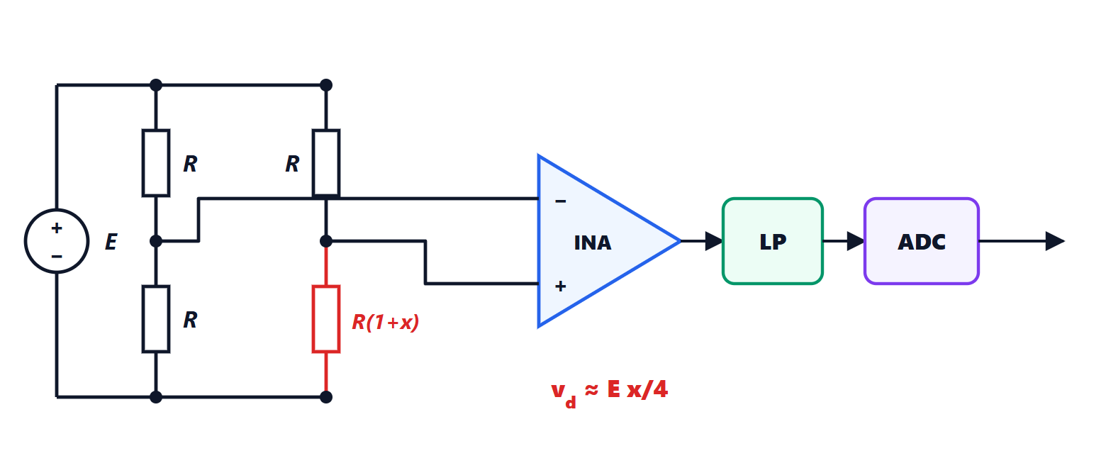
In a quarter bridge a single gauge replaces one of the four resistances, and the output is about  : with
 V,
 and 1000 µε it is 2.5 mV. The drawback is that temperature changes the gauge resistance just as a strain does, and the bridge cannot tell them apart.
Theorem (half bridge). If two gauges are mounted on the same side of the bridge, one in tension and one in compression,  below and
 above, and the other side has two equal resistances, the output is exactly

linear, twice that of the quarter bridge, and insensitive to temperature.
Proof. The side with the fixed resistances gives  . The side with the gauges is a divider with total resistance
 , independent of
 , so the voltage at its midpoint is
 . The difference is
 , with no approximation. A temperature change multiplies both gauges by the same factor
 : the divider ratio does not change and neither does the output. ∎
It is the natural configuration for a beam in bending, where the upper face stretches and the lower one shortens. With four active gauges (full bridge) the output doubles again, to  . The load cells in weighing scales are full bridges on a calibrated elastic element.
Thermocouples
Two wires of different metals welded at one end generate a small voltage that depends on the difference in temperature between the hot junction and the free ends (Seebeck effect):

For the type K thermocouple (nickel-chromium and nickel-aluminium), the most common one,  µV/°C, and it works up to more than 1200 °C. The practical consequence is that a thermocouple does not measure a temperature but a difference: the instrument must know the temperature of the cold ends, at its terminals, and add its contribution. This is cold-junction compensation, done with a temperature sensor next to the terminals. An error of 1 °C on the cold junction is an error of 1 °C on the measurement.
By the law of intermediate metals, the instrument’s copper wires do no harm as long as the two copper-thermocouple junctions are at the same temperature: that is why the terminals are mounted on an isothermal block. If the thermocouple must be extended, extension cables of the same metals are used. The voltages are small (41 µV per degree) and long cables pick up interference: low-offset amplifiers with good common-mode rejection are needed.
Pt100 resistance thermometers
Platinum has a resistance that increases with temperature in an almost linear and highly reproducible way. The Pt100 is 100 Ω at 0 °C, with coefficient  /°C:

(for the highest accuracy the Callendar-Van Dusen equation is used, with a small quadratic term). It is measured by passing a constant current, typically 1 mA, and reading the voltage: 0.385 mV per degree. Two errors must be kept under control:
- lead resistance: with two wires of 0.2 Ω each, the extra 0.4 Ω are worth about 1 °C. The three-wire connection is used, which compensates the leads if they are equal, or the four-wire one (lesson on resistance measurement), which eliminates them;
- self-heating: the current dissipates
 in the sensor and warms it. With 1 mA through 100 Ω it is 0.1 mW, usually negligible; with 10 mA it would be 10 mW and a few tenths of a degree in still air.
Pt100s are more accurate and stable than thermocouples but work over a narrower range, typically from −200 to 600 °C. NTC thermistors are much more sensitive (a few per cent per degree) but strongly non-linear, suited to limited ranges.
Conditioning: common mode and interference
The output of a bridge is a small differential signal on top of a large common-mode voltage: with V, the two bridge nodes are both around 2.5 V and differ by a few millivolts. An instrumentation amplifier (Applied Electronics lesson) with a high common-mode rejection ratio is needed.
Example. With a CMRR of 100 dB (i.e.  ), the 2.5 V of common mode produce an input-referred error of
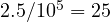 µV: 1 % of the 2.5 mV of the quarter bridge. With 80 dB the error would rise to 10 %.
The other precautions are those of good practice: twisted, shielded cables, with the shield grounded at one end only so as not to create ground loops, in which potential differences between the grounds of distant points drive currents; filters that cut mains interference and, before the converter, everything above half the sampling frequency; AC excitation or periodic polarity reversal to remove offsets and thermoelectric voltages.
The 4-20 mA current loop
In industrial plants sensors are tens or hundreds of metres away from the control system. Transmitting a voltage over such distances would mean losing accuracy to drops in the cables and to interference. A current is transmitted instead: the transmitter sets the current in the loop between 4 and 20 mA in proportion to the measured quantity,

and the receiver reads it as a voltage across a resistance (250 Ω give 1 to 5 V). The current is the same throughout the loop, so the cable resistance does not matter as long as the supply can overcome it. The live zero at 4 mA has two advantages: zero current signals a broken wire, distinguishing it from a reading at the minimum, and the 4 mA are enough to power the transmitter itself over just two wires. A digital communication (the HART protocol) can be superimposed on the analogue loop to configure and diagnose the sensor remotely.