The oscilloscope: bandwidth, rise time, sampling and probes
The digital oscilloscope and trigger, rise time 0.35/B with proof, sampling and aliasing, the compensated 10:1 probe with proof, common mistakes with grounding and capacitive loading.
The oscilloscope is the instrument that shows signals in time: waveforms, noise, delays, edges. It is also the instrument that most easily shows things that are not there, if its limits are not known. In this lesson we look at how a digital oscilloscope is built, the link between bandwidth and rise time with its proof, sampling, the compensated probe with the compensation condition proved, and the most common mistakes.
How a digital oscilloscope is built
Each channel has an attenuator and a vertical amplifier, which bring the signal to the right amplitude for the analogue-to-digital converter, almost always 8-bit, sampling at very high speed (gigasamples per second). The samples go into a memory, and a trigger circuit decides which portion of the signal to show: the one around the instant at which the signal crosses a given level with a given slope. Without a trigger a periodic signal would drift across the screen; with the trigger every acquisition starts from the same point of the waveform and the picture stands still.
The figures that characterise an instrument are the bandwidth, the sample rate, the memory depth (how many samples per acquisition) and the vertical resolution. With 8 bits the screen has 256 levels: at 1 V/division over 8 divisions the step is about 31 mV. So it pays to set the scale so that the signal fills almost the whole screen.
Bandwidth and rise time
The bandwidth is the frequency at which a sine wave is displayed with its amplitude reduced by 3 dB, i.e. to 71 %. Even below the bandwidth the error is not negligible: with a first-order response, a sine wave at one third of the bandwidth appears 5 % smaller. For digital signals, however, what matters is the rise time, the time needed to go from 10 % to 90 % of the final value.
Theorem. For a first-order system with bandwidth  , the rise time is

Proof. The step response is  , with bandwidth
 . 10 % is reached when
 , i.e.
 ; 90 % when
 , i.e.
 . The difference is
 , and substituting
 gives
 . ∎
A 100 MHz oscilloscope therefore has its own rise time of about 3.5 ns. When an edge is measured, the two times combine roughly in quadrature:

A true 5 ns edge appears as  ns: 22 % slower. The practical rule is to choose an instrument with a bandwidth 3 to 5 times higher than the highest frequency of interest, or with a rise time 3 to 5 times shorter than the edge to be measured.
Sampling
A digital oscilloscope must respect the sampling theorem (Signal Theory lesson): more than two samples per period of the highest component are needed, and in practice a sample rate of at least 2.5 times the bandwidth is required, preferably more to see the shape of the edges well. If the signal contains components above half the sample rate there is aliasing: a stable waveform appears on the screen, but at a false frequency.
The greatest danger is at slow timebases: with fixed memory, widening the window lowers the sample rate. An oscilloscope with 10 000 points of memory, set to 1 s for the whole screen, samples at only 10 kHz, and a disturbance at 9.99 kHz appears as a slow oscillation that does not exist. To find out, just change the timebase: a real signal stays the same, an alias changes frequency.
The compensated probe
Connecting a coaxial cable directly to the input adds tens of picofarads to the circuit under test. That is why the 10:1 probe is used: a resistance  MΩ in the tip forms a divider with the instrument input,
 MΩ. But the input also has a capacitance
 (instrument plus cable), and a resistive divider with a capacitor across only one of its resistances would not have the same ratio at all frequencies. So a capacitor
 is added across
 .
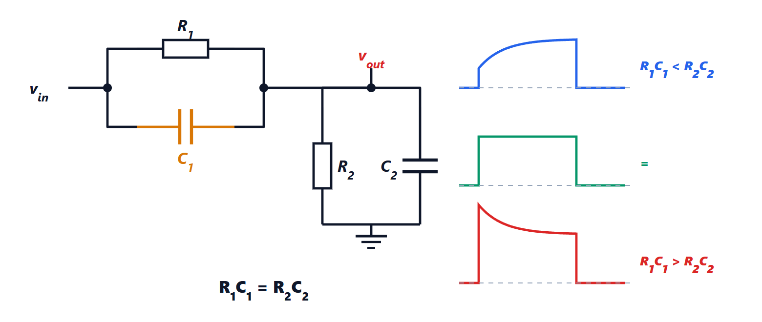
Theorem. The division ratio is the same at all frequencies if and only if  .
Proof. The impedances of the two parallel combinations are

and the ratio is  . We have
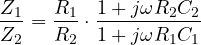
which is independent of  if and only if the two time constants are equal; it is then
 and the ratio is
 at every frequency. ∎
With  pF one needs
 pF. The circuit under test then sees 10 MΩ in parallel with the series of and , i.e. 9 pF: ten times better than the bare cable. Every probe has a small adjustable capacitor for compensation: the probe is connected to the oscilloscope’s square-wave output and adjusted until the edges are sharp and the flat parts are flat. An under-compensated probe rounds the edges and makes a fast signal look slow; an over-compensated one creates spikes that do not exist.
The most common mistakes
- The long ground lead. The 15 cm ground lead with its crocodile clip has an inductance of about 150 nH, which with the 10 pF of the probe resonates near 130 MHz: fake ringing appears on fast edges. For fast measurements the short ground spring on the tip is used.
- The oscilloscope ground is earthed. Connecting the clip to a point that is not at ground (for instance in a mains-powered circuit without a transformer) creates a short circuit to earth. Floating measurements need differential probes.
- Capacitive loading. Even 9 pF at 100 MHz is an impedance of about 180 Ω: on high-impedance circuits the probe changes the signal. For very fast signals active probes are used, with capacitance below one picofarad.
- AC coupling. In AC mode a series capacitor removes the DC component, but it also distorts slow square waves, whose flat parts appear tilted.