The two-stage CMOS op-amp and Miller compensation
Two-stage structure and gain, Miller compensation with the gain-bandwidth product proved, pole splitting and phase margin, the right-half-plane zero, cascode and gain boosting.
Inside almost every chip, even digital ones, there are analogue circuits: voltage references, converters, regulators, radio receivers. Their main building block is the integrated operational amplifier, designed with rules different from those of the discrete op-amp seen in Applied Electronics, because every transistor can be sized but intrinsic gains are low and parasitic capacitances are everywhere. In this lesson we look at the two-stage CMOS op-amp, its gain, Miller compensation with the proof of the gain-bandwidth product, the second pole and the phase margin, the right-half-plane zero and higher-gain circuits.
The two-stage op-amp
The most classic structure has:
- a differential first stage (Applied Electronics lesson on the differential pair): an input transistor pair with a current-mirror active load, converting the input voltage difference into current with transconductance
 into an output resistance
 ;
- a common-source second stage, with transconductance
 and output resistance
 , providing the rest of the gain and the output swing.
The DC gain is

With intrinsic gains  of 20-50 per stage in modern processes (lesson on the nanometre MOSFET), 60-70 dB is reached.
Miller compensation
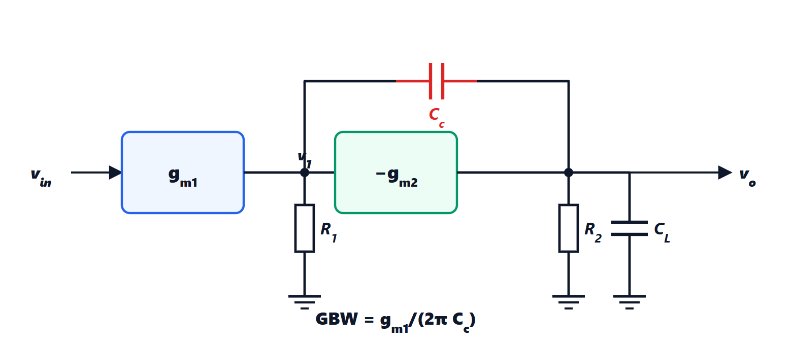
Each stage has a pole, and two close poles would give, in feedback, a poorly damped or unstable system. So a capacitor  is connected between the input and the output of the second stage. Because of the Miller effect, seen from the intermediate node the capacitor looks multiplied by the second stage’s gain,
 : a huge capacitance, which creates a low-frequency dominant pole.
Theorem. With Miller compensation the amplifier’s gain-bandwidth product is
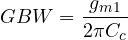
independent of the second stage and of the output resistances.
Proof. The dominant pole is at the intermediate node, with resistance and effective capacitance  (neglecting the 1 compared with the gain):
 . The gain-bandwidth product is the DC gain times the dominant pole frequency:

and dividing by  gives the formula in hertz. ∎
The result is convenient: the output resistances, which vary a lot with process and temperature, cancel, and the crossover frequency depends only on a transconductance and a capacitor, both well controlled. Example. With  mS and
 pF,
 MHz.
The second pole and phase margin
Compensation also has a less obvious effect: at high frequencies shorts the second stage, which behaves like a diode of conductance , and the second pole moves up, to about

(this is “pole splitting”). For the amplifier used as a follower to be stable with a good phase margin (lesson on the Nyquist criterion), the second pole must lie beyond the gain-bandwidth product: with  the margin is about 60°. The design rule follows:
 : the second stage must have a large transconductance, and therefore consume current, all the more the heavier the capacitive load.
The right-half-plane zero
Capacitor also offers a direct path from the intermediate node to the output, which at high frequencies carries the signal with the opposite sign to that of the second stage. This produces a right-half-plane zero at  , adding phase lag like that of the boost converter (Power Electronics lesson on converter control). It is moved or eliminated with a nulling resistor in series with , of value about
 , or by isolating the direct path with a follower.
Higher-gain amplifiers
When 60-70 dB is not enough, for instance in precision converters, the following are used:
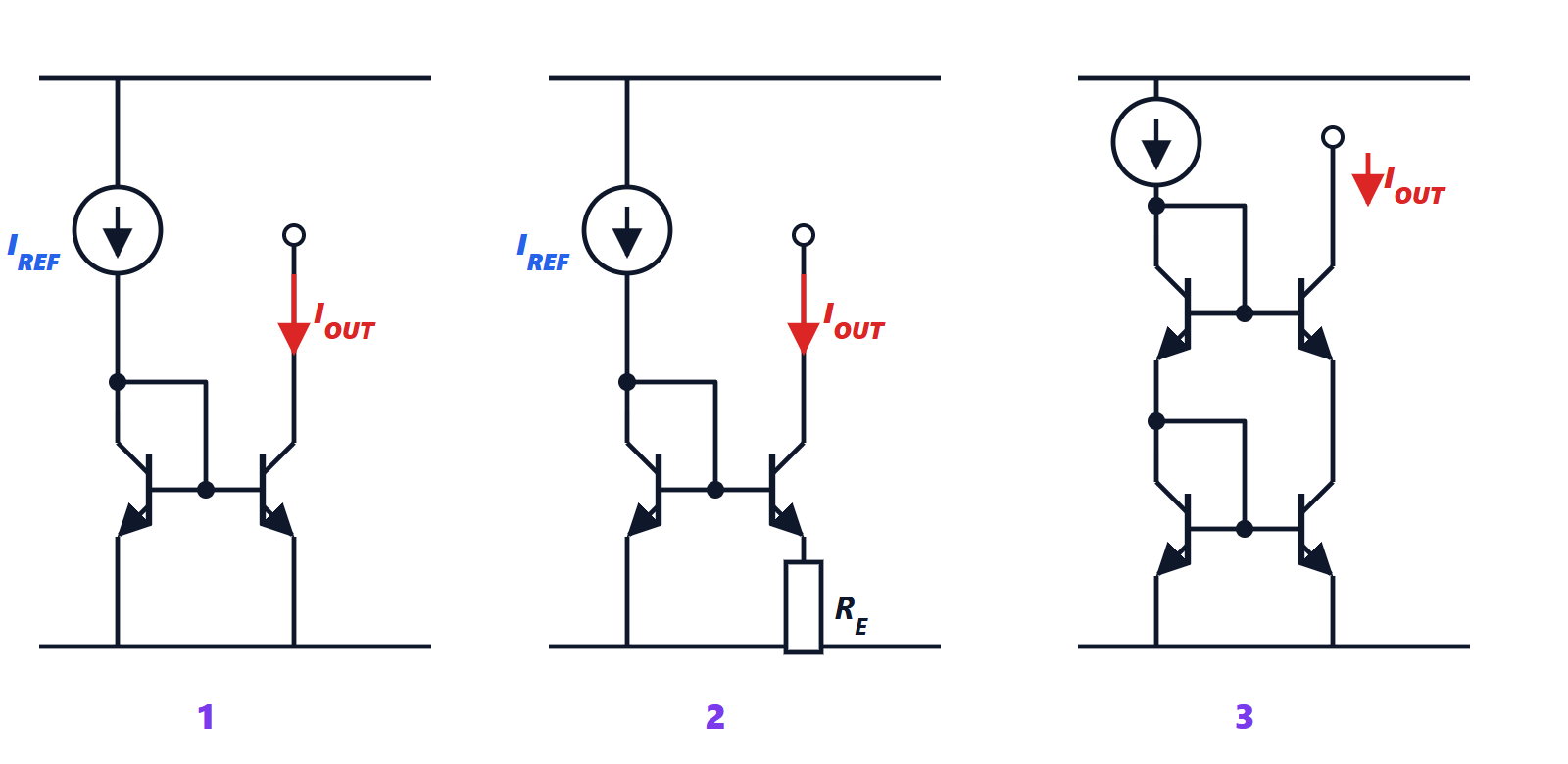
- the cascode (lesson on current mirrors): a series transistor that multiplies the output resistance by its intrinsic gain, bringing a single stage to 60 dB. The telescopic and folded-cascode op-amps thus achieve high gains with a single stage, compensated by the load capacitance itself, but they have a reduced output swing, because many series transistors use up voltage headroom;
- gain boosting: a small auxiliary amplifier that regulates the cascode, for gains of 100 dB and more.
With 0.8-1 V supplies the signal swing keeps shrinking, and analogue design in advanced processes has become a balancing act between gain, speed, noise and available voltages. Many functions then move into the digital domain, where small transistors are an advantage: this is the trend of oversampled converters with digital processing (Digital Signal Processing lesson on multirate processing).