Frequency and time measurement: counters, timebase and Allan variance
Direct counting and period counting, the plus or minus one count error, crossover frequency proved, reciprocal counters, timebase error, reference oscillators, Allan deviation, trigger error.
Frequency and time are the quantities measured with the highest accuracy of all: an atomic clock is off by less than a second in millions of years, and a laboratory counter reads ten or twelve significant digits. The reason is that counting is easy, and counting well is only a matter of having a good reference. In this lesson we look at the frequency counter and the period counter with their counting errors, the crossover between the two with its proof, the timebase error, reference oscillators and the Allan variance.
The direct-counting frequency meter
The principle is elementary: a gate is opened for an accurately known time  and the edges of the signal passing through are counted. If the signal has frequency
 , the count is about
 , and the instrument displays
 . The gate time is derived from an internal reference oscillator, by dividing its frequency.
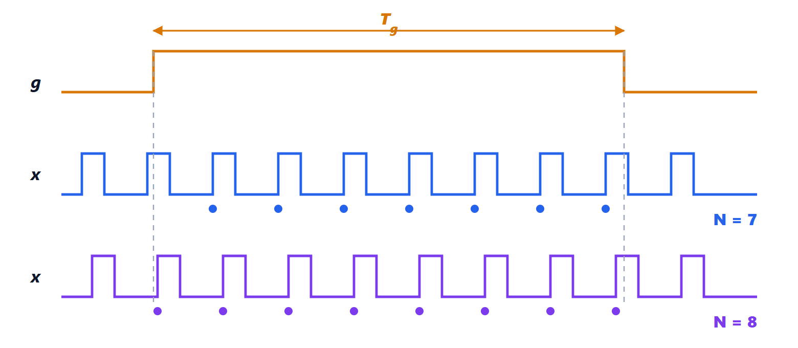
The gate is not synchronised with the signal, so depending on where the edges fall relative to the opening one edge more or one fewer is counted: this is the ±1 count error, and the relative error is
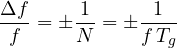
Example. With  s, a 10 MHz signal is read with a resolution of 1 Hz, i.e.
 ; a 1 kHz signal with a resolution of 1 Hz, i.e. 0.1 %. Direct counting is excellent for high frequencies and poor for low ones.
The period counter
For low frequencies the scheme is reversed: the signal opens the gate for one period  , and the pulses of the reference clock, of frequency
 , are counted. The count is
 and the ±1 count error is now
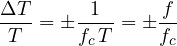
This time the error grows with frequency. With  MHz, a 1 kHz signal is measured with an error of
 , a hundred times better than direct counting with a 1 s gate.
Theorem. Direct counting with gate and the period counter with clock have the same error at the frequency

Below  the period counter is better, above it direct counting.
Proof. Equate the relative errors:  , i.e.
 . The first error decreases with , the second increases, so to the left of the crossing point the second is smaller and to the right the first. ∎
With MHz and s,  kHz, where both are off by about
 . Modern reciprocal counters remove the problem: they open the gate in sync with an edge of the signal, count the signal periods and the clock periods together, and compute the ratio. The resolution then depends only on the clock and on the measurement time, not on the frequency; with interpolation of the time between edges, resolutions of tens of picoseconds per measurement are reached.
The timebase error
The count is perfect to within one unit, but the gate time comes from the internal oscillator, which has its own error.
Theorem. If the reference frequency has a relative error  , the measured frequency has the same relative error .
Proof. The gate time is obtained by counting  periods of the reference:
 . If the reference is
 , the gate lasts
 ,
 edges are counted, and the instrument, which divides by the nominal , displays
 . The relative error has magnitude . The same holds for the period counter, where
 appears directly. ∎
So the timebase sets a limit that no gate time can beat. Typical choices are:
- plain crystal (XO):
 , varies a lot with temperature;
- temperature-compensated crystal (TCXO):
 , the one in many inexpensive instruments and in phones;
- oven-controlled crystal (OCXO):
 per year, with excellent short-term stability;
- rubidium:
 per year, a compact atomic clock;
- GPS-disciplined oscillator (GPSDO): an OCXO or a rubidium continuously corrected by the satellite signals, which carry the time of caesium clocks, with an average error below
 .
Laboratories distribute a common 10 MHz reference to all instruments, which have a dedicated input: in this way all the frequency measurements on the bench share the same accuracy.
Stability and the Allan variance
Accuracy says how far the mean frequency is from the nominal one; stability says how much the frequency fluctuates over time. To describe it the ordinary standard deviation is not used: oscillator noise contains low-frequency components (flicker noise and random walk) for which the standard deviation keeps growing with the measurement duration and does not converge. The Allan deviation is used instead: the mean relative frequencies  are measured over consecutive intervals of duration
 , and one computes
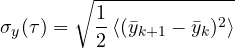
i.e. only the difference between adjacent measurements is considered, which is insensitive to slow drifts. The plot of  against tells for which averaging time an oscillator is most stable: an OCXO reaches around one second, then gets worse because of ageing; a hydrogen maser goes down to
 in a day.
Time-interval measurements
A counter also measures the time between two events: an edge on one channel starts the count, an edge on the other stops it. Besides the quantisation error there is the trigger error: noise shifts the instant at which the signal crosses the threshold. Linearising the edge around the threshold, noise of RMS value  on an edge with slope
 produces a timing error

That is why the trigger is set at the steepest point of the edge and signals with fast edges are used: 1 mV of noise on a 1 V/ns edge shifts the instant by 1 ps, on a 1 V/µs edge by 1 ns. It is the same mechanism that produces jitter in digital systems and converters.