The digital voltmeter: dual slope, mains rejection and specifications
Structure of a multimeter, the dual-slope converter with proof, mains rejection and NPLC, digits and counts, quantisation uncertainty, real specifications and autozero.
The digital voltmeter is the heart of every bench multimeter: it measures DC voltages with six or more digits, and current, resistance and temperature measurements are built on it. In this lesson we look at the dual-slope converter, why its accuracy does not depend on its components, how it rejects mains interference, and how digits, counts and specifications are read. Converters in general (SAR, flash, sigma-delta) are covered in the Applied Electronics lesson on converters.
The structure of a digital voltmeter
The signal goes through an input divider that selects the range, a high-impedance amplifier, an analogue-to-digital converter and logic that corrects offset and gain with the calibration constants and displays the result. On the low ranges the input can exceed 10 GΩ; on the high ranges the divider brings the impedance to about 10 MΩ, the value to use in loading-effect calculations (lesson on voltmeters and ammeters).
The converter of precision multimeters is almost always integrating: it does not take a snapshot of the signal at one instant, but averages it over an interval. The most classic one is the dual-slope converter.
The dual-slope converter
An integrator (an op-amp with a capacitor in the feedback path, lesson on the integrator) works in two phases:
- for a fixed time
 , where
 is the clock period, it integrates the unknown voltage
 : the output ramps down with a slope proportional to ;
- then the input is switched to a reference voltage
 of opposite sign, and the output ramps up with a fixed slope. A counter measures the time
 needed to return to zero.
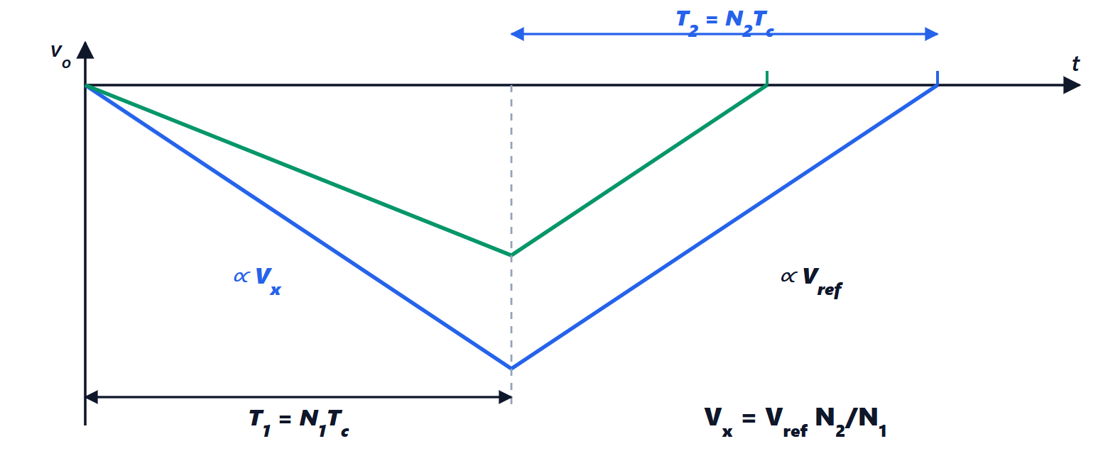
Theorem.  .
Proof. With resistance  and capacitance
 , at the end of the first phase the output is
 . In the second phase it rises with slope
 and returns to zero after
 , so
 .
 cancels:
 . Finally
 : the clock period cancels too. ∎
This is the merit of the method: neither , nor , nor the clock frequency appears in the result, as long as they stay constant during the conversion (a few milliseconds). The accuracy depends only on the voltage reference and on the count. With  counts one gets a 4½-digit voltmeter from inexpensive components.
Mains rejection
The leads pick up 50 Hz mains interference, which adds to the DC voltage being measured. The integrator attenuates it by itself, if  is chosen well.
Theorem. A sinusoidal disturbance of amplitude  and frequency
 produces, in the average over , an error of at most
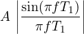
which vanishes when is an integer multiple of the period  .
Proof. The average over of  is

With the identity  the numerator is
 , whose magnitude is at most
 over the unknown phase
 . Dividing by
 gives the bound. If
 is an integer,
 . ∎
With  ms the 50 Hz disturbance and all its harmonics cancel; with
 ms both 50 and 60 Hz cancel, and the instrument works in Europe and America alike. That is why bench multimeters express the integration time in NPLC (number of power-line cycles): 1 NPLC is the minimum that rejects the mains, 10 or 100 NPLC reduce noise at the expense of speed. White noise in the average decreases as
 , like the mean of
 readings in the lesson on uncertainty.
Digits, counts and resolution
A 3½-digit display shows up to 1999: three full digits plus a leading “half” digit that can only be 0 or 1. A 4½-digit one goes to 19 999, a 6½-digit one to 1 999 999. Nowadays the number of counts is often given: a “6000-count” meter shows up to 5999. The resolution is the value of the last digit: on the 2 V range of a 3½-digit meter it is 1 mV.
Quantisation adds an uncertainty: the true value can be anywhere within half a digit of the reading. With the uniform distribution over  , where
 is the step, one gets
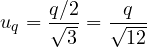
the same result as the quantisation noise in the Signal Theory lesson on quantisation.
Real specifications
A 6½-digit bench multimeter has, on the 10 V range, specifications of the order of ±(0.0035 % of reading + 0.0005 % of range) one year after calibration. The items to look at are:
- 24-hour, 90-day and one-year accuracy: the drift of the reference makes the error grow over time;
- temperature coefficient: added outside the calibration interval, typically 23 ± 5 °C;
- input impedance and bias current: with high-impedance sources they matter more than the digits;
- normal-mode (NMRR) and common-mode (CMRR) rejection, in dB at the mains frequency.
The best instruments perform autozero: between measurements they short the input, measure the offset and subtract it, removing the amplifier drift. Thermoelectric voltages at contacts between different metals (a few microvolts per degree) remain a limit for microvolt measurements: pure copper leads are used and the measurements with reversed polarity are averaged.