Voltmeters and ammeters: loading effect, shunts and RMS value

The voltmeter and the ammeter are the first instruments one uses and the first one gets wrong, not because they are inaccurate but because connecting them changes the circuit. In this lesson we look at how they are connected, the loading effect with its proof, how the range of an instrument is extended with shunts and series multipliers, and why a cheap multimeter can be 11 % off on a square wave.

How they are connected

The voltmeter measures the potential difference between two points and is connected in parallel: ideally it draws no current, i.e. its internal resistance is infinite. The ammeter measures the current in a branch and is connected in series, opening the branch: ideally it causes no voltage drop, i.e. its internal resistance is zero. A real instrument is modelled as the ideal one plus its internal resistance, and all insertion errors come from there.

A classic and dangerous mistake: connecting an ammeter in parallel with a source. Its almost-zero resistance turns it into a short circuit; that is why multimeters have a fuse on the current input.

The voltmeter loading effect

Any linear circuit, seen from the two measurement points, reduces to its Thévenin equivalent: a voltage in series with a resistance (Electrical Engineering lesson on Thévenin and Norton).

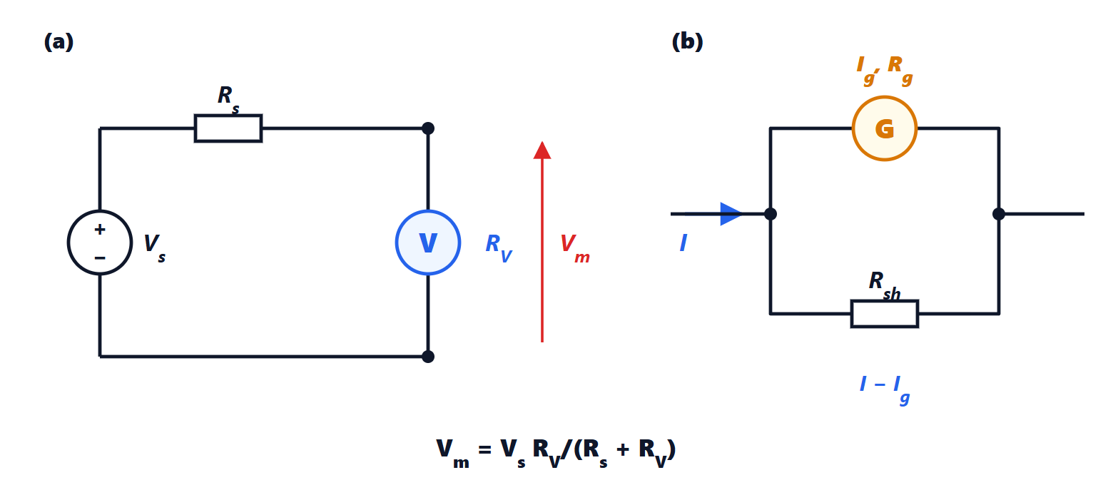
Theorem. The voltmeter reads

Proof. The voltmeter closes the circuit: the current flows through and in series, and the voltage across is that of the divider. The relative error follows by subtracting and dividing; for the denominator is about . ∎

The error is always negative: the voltmeter reads low. It is a systematic error, and if and are known it can be corrected.

Example. An old 20 kΩ/V moving-coil meter on the 10 V range has kΩ. On a point with kΩ (the middle of a 100 kΩ + 100 kΩ divider) it reads of the true value: −20 %. A digital multimeter with MΩ is about −0.5 % off. On high-impedance circuits, such as a MOSFET gate or a pH electrode, electrometers with of Ω and more are needed.

The ammeter loading effect

Inserting an ammeter in a branch adds its in series. By the same reasoning, if the branch sees a Thévenin resistance , the current becomes

Multimeter makers specify the burden voltage: the drop across the instrument at full scale. A multimeter with a 0.2 V drop on the 200 mA range has Ω: in a circuit supplied at 3.3 V through 100 Ω the error is 1 %. To measure currents without opening the circuit, clamp meters are used, sensing the magnetic field of the conductor (Hall effect for DC, transformer for AC).

Extending the range: shunts and multipliers

The basic analogue instrument is the galvanometer: a moving coil in a magnetic field, deflecting in proportion to the current and reaching full scale with a small current (typically 50 µA), with its own resistance .

Theorem (shunt). To measure currents up to , the following resistance is placed in parallel with the galvanometer:

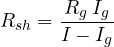
Proof. Galvanometer and shunt are in parallel, so they have the same voltage. At full scale flows in the galvanometer and the rest, , in the shunt: , which gives the formula. ∎

With µA and kΩ, a 1 A range needs Ω. Likewise, to turn it into a 10 V voltmeter a series multiplier kΩ is added. The ratio kΩ/V is the instrument’s sensitivity, the number printed on the dials of old analogue testers. Digital multimeters do the same thing the other way round: they always measure a voltage, and for currents they read it across an internal shunt.

Mean value, RMS value and form factor

In AC one almost always wants the RMS value, the one that gives the same power in a resistor (Electrical Engineering lesson on power):

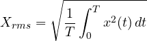
Cheap instruments, however, rectify the signal and measure the mean value of its magnitude, then multiply by the form factor of the sine wave, .

Theorem. For a sine wave the form factor is .

Proof. For the RMS value is . The mean of the magnitude over half a period is

and the ratio is . ∎

The instrument is right only for sine waves. With a square wave of amplitude the mean magnitude is and the RMS value is also : the instrument shows , +11 %. With a triangle wave the mean magnitude is and the RMS value : the instrument shows , −3.8 %. With the heavily distorted currents of electronic power supplies the errors easily exceed 30 %.

True RMS instruments really compute the root of the mean of the square, with a dedicated circuit or numerically on the samples. They have two stated limits: the bandwidth and the maximum crest factor, the ratio of peak to RMS value they can handle without saturating (typically 3).

Reading the specifications

Multimeter specifications are written as ±(% of reading + digits): the first part is a gain error, the second an offset error expressed in units of the last digit. Two consequences follow:

• use the lowest possible range, because the fixed digits weigh less on a large reading;
• resolution and accuracy are different things: a six-digit display does not guarantee six correct digits.

The specifications hold within a temperature interval (usually 23 ± 5 °C) and for a certain time after calibration; outside it a temperature coefficient is added. From the specifications the Type B uncertainty is derived with the uniform distribution, as in the lesson on uncertainty.