Measurement uncertainty: errors, Type A and Type B, propagation
Systematic and random errors, uncertainty of the mean with proof, the uniform distribution and Type B uncertainty, the propagation law proved, expanded uncertainty, writing the result and traceability.
To measure is to compare a quantity with a standard and to state not only a number, but also how far that number can be trusted. A result without uncertainty is not a measurement result: “the resistance is 500 Ω” does not say whether we can tell it apart from one of 501 Ω. In this lesson we look at systematic and random errors, the two ways of evaluating uncertainty (Type A and Type B), the propagation law with its proof and the correct way to write a result.
Measurand, error and uncertainty
The measurand is the quantity to be measured, for instance the voltage across a resistor under precise conditions. Its true value cannot be known: every measurement approximates it. The difference between the measured value and the true one is the error, which therefore is not known either. What is known is the uncertainty: a parameter describing the width of the interval in which the value of the measurand can reasonably be believed to lie.
Errors fall into two families:
- systematic: they repeat identically at every measurement (an instrument out of calibration, the loading effect of a voltmeter, the resistance of the leads). Repeating the measurement does not reduce them; they are corrected when known and their residual uncertainty is estimated;
- random: they change from one reading to the next (noise, small changes in the environment). They are reduced by averaging several readings.
The international vocabulary distinguishes trueness (how close the mean is to the true value: it concerns systematic errors) from precision (how close the readings are to one another: it concerns random ones). Accuracy covers both.
Type A uncertainty: from the statistics of the readings
We take  independent readings
 . The best estimate is the mean, and the spread is measured by the experimental standard deviation:

Theorem. The standard uncertainty of the mean is  .
Proof. The readings are independent random variables with the same variance  . The variance of a sum of independent variables is the sum of the variances, and multiplying by a constant
 multiplies the variance by
 . Hence

and estimating  with
 gives . ∎
The practical consequence: halving the random uncertainty takes four times as many readings. Beyond a certain point it is no longer worth it, because the systematic part dominates and averaging does not touch it.
Type B uncertainty: from the available information
When the measurement is not repeated, the uncertainty is derived from other information: the manufacturer’s specifications, the calibration certificate, the display resolution. Often all we know is that the error lies within an interval  , with no preferred value: a uniform distribution is then assumed.
Theorem. For a uniform distribution on  the standard uncertainty is
 .
Proof. The density is  in the interval and the mean is zero, so

whence . ∎
Example. A multimeter specifies ±(0.05 % of reading + 2 digits) on the 6 V range with 1 mV resolution. Reading 5.000 V the limit is  mV, and the standard uncertainty is
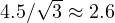 mV.
Propagation of uncertainty
The measurand is hardly ever measured directly: it is computed from other quantities,  . How do their uncertainties combine?
Theorem (propagation law). If the input quantities are independent and the uncertainties small,
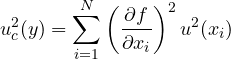
Proof. For small variations  is expanded to first order around the estimated values:
 , with
 (the sensitivity coefficients). The variance of a linear combination of independent variables is
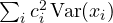 , as in the previous proof. Replacing the variances by the squared uncertainties gives the formula. ∎
Two special cases are used all the time:
- for a sum or difference
 the absolute uncertainties add in quadrature:
 ;
- for a product or quotient
 or
 the relative uncertainties add in quadrature:
 . Just compute the derivatives and divide by
 .
The sum in quadrature is always smaller than the plain sum: two independent errors are unlikely to be both at their maximum and with the same sign. If instead the quantities are correlated (for instance measured with the same miscalibrated instrument), the formula must be completed with the covariance terms.
Example. A resistance is measured with the voltmeter-ammeter method:  V with relative uncertainty 0.10 %,
 mA with relative uncertainty 0.20 %. Then
 Ω and

The current weighs more: to improve the measurement a better ammeter is needed, not a better voltmeter. This is the real use of an uncertainty budget: it tells you where to invest.
Expanded uncertainty and writing the result
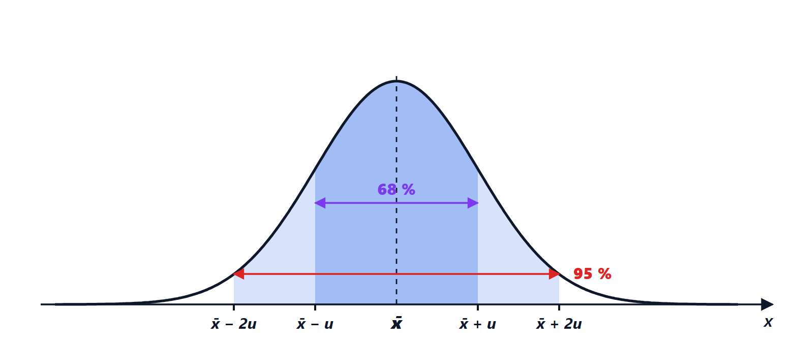
The standard uncertainty corresponds to one standard deviation. If the distribution of the result is roughly Gaussian, the interval  contains the value with a probability of about 68 %. For safer statements the expanded uncertainty
 is used, with coverage factor
 , corresponding to about 95 %.
The result is written like this:  with . The practical rules:
- the uncertainty is rounded to one or two significant figures: writing 2.183 Ω means claiming to know the uncertainty of the uncertainty;
- the value is rounded to the same decimal place as the uncertainty;
- the coverage factor or confidence level is always stated.
Calibration and traceability
An instrument is reliable only if it has been compared with a better standard, and that one with an even better one, up to the national standards of the SI units (kept by national metrology institutes such as NIST, PTB, NPL or INRiM). This unbroken chain of calibrations, each with its stated uncertainty, is metrological traceability. The calibration certificate gives the corrections to apply and their uncertainty, which enters the budget as a Type B contribution. That is why instruments in laboratories carry a label with the date of the next calibration: after that date the specifications are no longer guaranteed.