Power measurement: wattmeter, two-wattmeter method and distorted waveforms
Electrodynamic and digital wattmeters, Blondel's theorem, the two-wattmeter method with proof, readings with a balanced load and reactive power, harmonics, power factor and THD, energy meters.
Electrical power is the quantity that appears on the electricity bill and that decides how hot components get, and it is also one of the easiest to measure wrongly. Multiplying RMS voltage and current is not enough: the mean of the instantaneous product is needed. In this lesson we look at the wattmeter, measurement in three-phase systems with the two-wattmeter (Aron) method and its proof, and what changes when waveforms are not sinusoidal. The definitions of active, reactive and apparent power are in the Electrical Engineering lesson on power.
What is measured
Active power is the mean of the instantaneous power over a period:
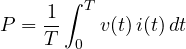
In sinusoidal steady state it is  , with
 and
 RMS values. A voltmeter and an ammeter give only the apparent power
 ; for the active power an instrument that multiplies instantaneous values, i.e. one that “sees” the phase shift, is needed.
The wattmeter
The wattmeter has two circuits: a current circuit, in series with the load, carrying the current, and a voltage circuit, in parallel, supplied by the voltage. In the classic electrodynamic instrument the fixed coil carries the current and the moving coil a current proportional to the voltage: the torque is proportional to the instantaneous product, and the inertia of the moving part averages it. The instrument thus reads  directly.
Modern wattmeters are digital: they sample voltage and current with two simultaneous converters and compute
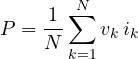
over an integer number of periods, synchronising the sampling with the mains. From the same samples they also derive the RMS values, the apparent power, the power factor and the harmonics.
Like voltmeters and ammeters, the wattmeter has an insertion error: the voltage circuit can be connected upstream or downstream of the current circuit, and the power drawn by the instrument adds to that of the load. The reasoning is the same as for the voltmeter-ammeter method (lesson on resistance measurement): with low-impedance loads connect the voltage circuit downstream, with high-impedance loads upstream. The current and voltage ratings must also be respected, not only the power range: with a low power factor load the instrument can be over-current while the pointer shows little.
Three-phase systems and Blondel’s theorem
In an  -wire system the total power is measured with
 wattmeters (Blondel’s theorem): each carries the current of one wire and the voltage between that wire and a common wire chosen as reference, which needs no wattmeter. With the neutral (four wires) three wattmeters are needed; without neutral (three wires) two are enough: this is the two-wattmeter method, also called the Aron connection.
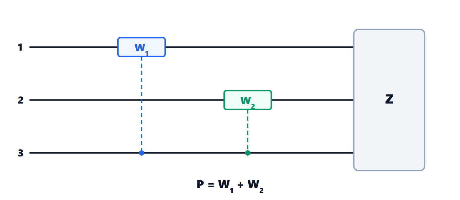
Theorem (two-wattmeter method). In a three-phase system without neutral, whatever the load (balanced or not), the total active power is  , with
 measuring
 and
 ,
 measuring
 and
 .
Proof. Take the voltages of the three wires with respect to any point. The instantaneous power entering the load is  . Without neutral the three currents sum to zero (Kirchhoff’s current law applied to the load), so
 . Substituting:

Averaging over a period, each term is exactly the reading of one of the two wattmeters. No assumption was made about the load or the waveform. ∎
Readings with a balanced load
With a symmetrical set of voltages in positive sequence 1-2-3, line voltage , line current and a balanced load with phase angle  (positive if inductive), the two wattmeters read

Proof. With phase voltages  ,
 ,
 , the current
 lags
 by . The voltage
 has magnitude
 and phase
 , so the phase difference between
 and is
 . Likewise
 has phase
 and
 has phase
 : the phase difference is
 . A wattmeter reads the product of the RMS values times the cosine of the phase difference. ∎
Two useful results follow:
- the sum
 , the three-phase power, as it must be;
- the difference
 , so the reactive power is
 and the power factor follows from
 .
With a purely resistive load the two wattmeters read the same. When exceeds 60° (power factor below 0.5) becomes negative: an analogue instrument goes off scale backwards, and its voltage circuit must be reversed and the reading subtracted.
Distorted waveforms
Electronic power supplies, inverters and LED lamps draw currents very different from a sine wave. Expanding voltage and current in Fourier series (lesson on the Fourier transform) gives an important result.
Theorem. The active power is the sum of the contributions of the individual harmonics:

with  ,
 the RMS values of harmonic and
 their phase difference.
Proof. The product  contains terms of the form
 . For
 their mean over a period is zero, by the orthogonality of trigonometric functions; for
 the mean is
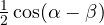 for the peak amplitudes, i.e.
 with RMS values. Only the sum of the terms at the same frequency remains. ∎
The consequence: if the mains voltage is sinusoidal, only the fundamental harmonic of the current carries active power, while the others increase the RMS current (and therefore the losses in the cables) without carrying energy. The power factor  no longer equals
 :

where the total harmonic distortion  is the ratio of the RMS value of the harmonics to that of the fundamental. A rectifier with a smoothing capacitor, with 100 % THD, has
 even with the fundamental in phase. That is why standards require power factor correction in power supplies above a few tens of watts, and measuring these loads needs digital wattmeters with a bandwidth of a few kilohertz.
Energy meters
Energy is the integral of power over time, in kilowatt-hours. Electronic household meters are digital wattmeters with an integrator: they sample voltage and current (the current with a shunt or a transformer), compute the power and accumulate the energy, distinguishing time bands and transmitting the data remotely. Their accuracy class, typically 1 %, is set by the standards for billing meters.