PID tuning for processes: direct synthesis, IMC and SIMC rules
Forms of the industrial PID, direct synthesis for the process with dead time with proof, choosing lambda, the SIMC correction with proof of the damping, derivative action, comparison with Ziegler-Nichols.
Once the process model is known, the PID controller can be tuned by reasoning rather than by trial and error. In this lesson we derive the direct synthesis tuning rules (related to IMC, internal model control) for the first-order-plus-dead-time process, with proof; we look at the SIMC correction for slow processes with the proof of the damping, and at how to choose the only remaining parameter, the desired closed-loop time constant. The Ziegler-Nichols rules, the PID structure and anti-windup are in the Automatic Control lesson on the PID.
The forms of the PID
In industrial controllers the PID is almost always written in the standard form (also called ISA):

with gain  , integral time
 and derivative time
 . Some manufacturers use the proportional band
 in per cent, or repeats per minute
 ; others the “series” form, with the parameters related differently. Before entering computed numbers one must know which form one’s controller uses. In practice the derivative is computed on the measurement rather than on the error (so as not to kick the valve at every set-point change) and is always filtered.
Direct synthesis
The idea is to choose the desired closed-loop response and derive the controller from it. For a process with dead time no controller can remove the delay, so the reasonable request is
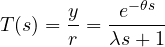
i.e. a first-order response with time constant  , delayed by
 . The parameter is our choice: small for a fast loop, large for a slow and robust one.
Theorem. For the process  , direct synthesis with the approximation
 gives a PI controller with

Proof. In closed loop  , whence
 . Substituting:

With the denominator becomes  , and

which is a PI in standard form with the parameters stated. ∎
The controller cancels the pole of the process with its zero ( ) and its gain is lower the longer the delay. It is an intuitive result: the slower the process is to respond, the more patient the controller must be.
Choosing lambda
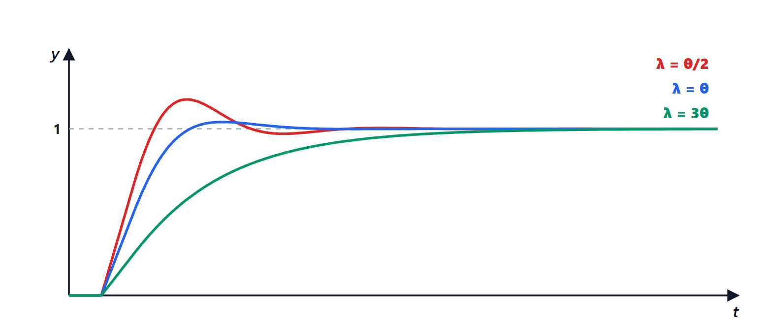
The recommended choice is  : it gives a fast response without oscillations, with a gain margin of about 3 and a phase margin of about 60°. A model identified from a step test has errors of 20-30 % in its parameters, and these margins tolerate them. Smaller values make the loop aggressive and sensitive to model errors; larger values, up to
 and beyond, are used when a quiet valve matters more than speed, for instance for the levels of surge tanks.
Example. For the heat exchanger of the previous lesson,  °C/%,
 s,
 s. With
 s:

The SIMC correction for slow processes
If the process is very slow ( ), cancelling its pole has a drawback: a disturbance entering at the process input, such as a change in steam pressure, is recovered with the slowness of
 , because the cancelled pole remains in the disturbance response. The SIMC rules (Skogestad) correct the integral time:

The factor 4 is not arbitrary.
Theorem. For an integrating process  (the limit of a slow process) controlled by a PI with
 and
 , neglecting the delay, the closed loop has damping
 .
Proof. The characteristic equation  , multiplied by
 , becomes
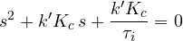
Comparing with  :
 and
 , so
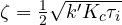 . With the given values
 , and
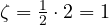 : critical damping, the fastest response without oscillation. A smaller would give
 and oscillations. ∎
The gain rule is consistent with the first-order one: an integrating process is the limit of  with and
 growing together,
 , and then
 tends exactly to
 .
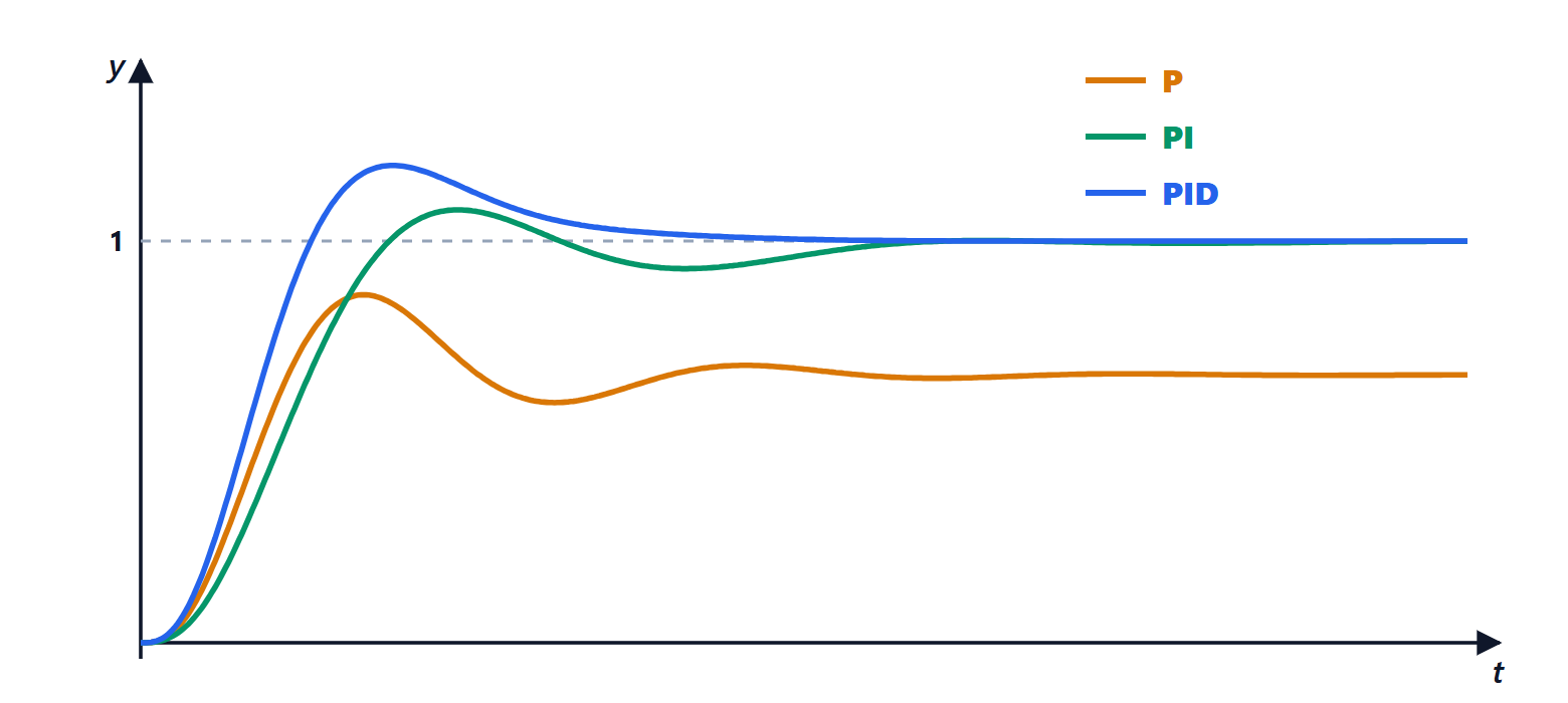
When derivative action is needed
For a first-order-plus-dead-time process a PI is enough: derivative action adds little and amplifies measurement noise. If the process has a second significant time constant  (model
 ), the same direct synthesis gives a series-form PID with
 : the derivative cancels the second pole. This is the typical case of temperatures, where the slowness of the process adds to that of the probe in its thermowell. For pressures and flows, fast and noisy, the derivative is hardly ever used.
Comparison with the classic rules
The Ziegler-Nichols rules aim at quarter-amplitude damping: each oscillation is a quarter of the previous one. It is an aggressive response, with overshoots close to 50 %, acceptable for a disturbance but not for today’s valves and plants. The direct synthesis and SIMC rules have a single parameter with a clear meaning, the desired speed, and allow a conscious choice between quickness and robustness. In plant practice the sequence is: step test, FOPDT model, tuning with , closed-loop check with a small set-point change, adjustment of if needed.