Modulation: AM, FM, QAM and Shannon capacity
Amplitude modulation and its spectrum, FM and Carson's rule, digital modulations and QAM constellations, OFDM, Shannon channel capacity with examples and the −1.6 dB limit.
An audio signal cannot be sent directly by radio: it would need antennas kilometres long, and every station would use the same frequencies. Modulation moves the signal around a chosen carrier frequency, where the antenna is small and there is room for many channels side by side. In this lesson we cover the analogue modulations AM and FM, digital modulations and the theoretical limit on the speed of any transmission: Shannon capacity.
Amplitude modulation
A message  , with bandwidth
 and
 , modulates the amplitude of a carrier at frequency
 :

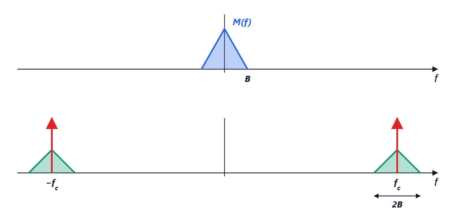
The spectrum. By the modulation property, multiplying by  shifts the spectrum by
 and halves it:
 . So the AM spectrum contains the carrier (a line at ) and two sidebands, copies of the message spectrum above and below the carrier. The occupied bandwidth is

AM’s strength is the receiver: with  the signal’s envelope is exactly
 , and it can be recovered with a diode, a capacitor and a resistor (the envelope detector, the same circuit as the rectifier with filter). Its weakness is efficiency: with a sinusoidal message and
 two thirds of the power goes into the carrier, which carries no information, and with real signals the share is even higher. More efficient variants remove the carrier (DSB) or also one of the two sidebands, which are redundant (SSB, used by radio amateurs), at the cost of a more complex receiver.
Frequency modulation
In FM the amplitude is constant and the message changes the instantaneous frequency:  , where
 is the peak deviation. The occupied bandwidth is well approximated by Carson’s rule:

Example. FM broadcast radio uses  kHz for 15 kHz audio:
 kHz, and indeed stations are spaced 200 kHz apart.
FM occupies much more bandwidth than AM, but in return it is much more robust to noise: disturbances mostly alter the amplitude, which the receiver ignores. It is the trade-off between bandwidth and quality that we will meet again in Shannon’s formula.
Digital modulations
To send bits, the carrier is modulated with a finite set of waveforms, the symbols. Each symbol is represented as a point in the plane of the two components  (in phase,
 ) and
 (quadrature,
 ):
 . The set of points is the constellation.
- ASK (on-off): carrier on or off; very simple, used in remote controls.
- FSK: two different frequencies for 0 and 1; robust, used in Bluetooth Low Energy.
- PSK: the carrier phase; BPSK carries 1 bit per symbol, QPSK 2 bits with four phases.
- QAM: amplitude and phase together; 16-QAM carries 4 bits per symbol, 256-QAM 8, 4096-QAM (Wi-Fi 7) 12.
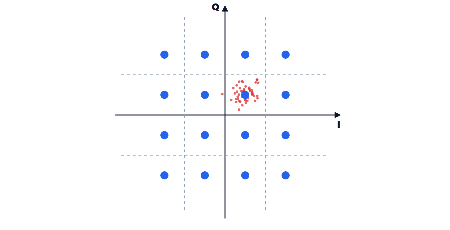
More points mean more bits per symbol, but points closer together for the same power: a higher SNR is needed so that noise does not move the received point into a neighbour’s region. That is why Wi-Fi and 5G keep switching constellation: 256-QAM close to the router, QPSK far away.
OFDM. Modern systems (Wi-Fi, 4G, 5G, DVB-T) split the band into hundreds or thousands of narrow subcarriers, each QAM-modulated, generated and separated with the FFT (Numerical Analysis lesson). Each subcarrier is so narrow that, for it, the channel is almost flat: echoes and intersymbol interference are avoided.
Shannon capacity
What is the maximum number of bits per second that can be sent, error-free, over a channel of bandwidth with white Gaussian noise?
Theorem (Shannon, 1948). The channel capacity is

Below this rate there exist codes that make the error probability as small as desired; above it, it is impossible. The theorem does not say how to build those codes: it took fifty years to get, with turbo codes and LDPC, within a few tenths of a decibel of the limit.
Examples.
- An analogue telephone line, 3 kHz bandwidth and 30 dB SNR:
 kbit/s. The modems of the 1990s reached 33.6 kbit/s, practically at the limit.
- A 20 MHz channel with 30 dB SNR:
 Mbit/s.
Bandwidth and power. Capacity grows in proportion to bandwidth, but only logarithmically with SNR: at high SNR, doubling the power adds just bit/s. With limited power and plenty of bandwidth there is an absolute limit: no system can work with  below
 , that is −1.6 dB. Space probes, with very little received power, work close to this limit; cellular systems, with little bandwidth and many users, rely instead on dense constellations and on multiple antennas (MIMO), which multiply capacity by creating several parallel channels in the same space.