ACC 6: from acceleration request to torque, powertrain, brakes and three zones
Forces on the vehicle with grade and wind, equivalent mass proved, inverse model and PI with anti-windup, three zones powertrain, coast and brakes, grade and mass estimation, hold on a climb.
https://www.electronics-engineering.com/en/acc-torque-control-powertrain-brakes-three-zones-grade-mass/
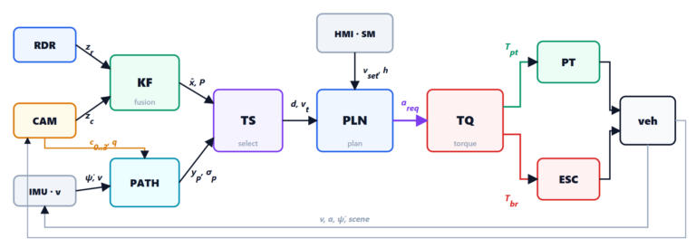
The planner requests an acceleration,  . The car, however, has no acceleration command: it has an engine (or an electric motor) that gives positive torque and a small braking torque when the pedal is released, and brakes that give only braking torque. Longitudinal control turns into two wheel torque requests,
 to the powertrain and
 to the ESC, taking into account grade, wind, payload and actuator delays. It is the point where vehicle physics really enters the software, and it is the part where you can feel an ACC: an abrupt change between engine and brakes, braking that comes late, a car that rolls back uphill.
The forces on the vehicle
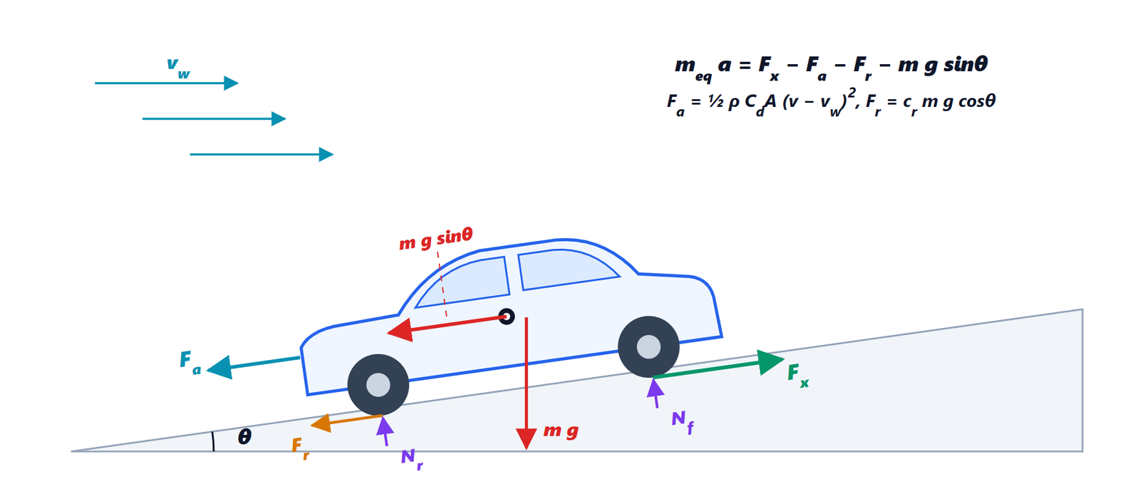
 with wind
 . Along the road act the driving force at the wheels
 , the aerodynamic drag
 , the rolling resistance
 and the weight component
 ; the normal reactions
 ,
 balance
 .
Newton’s second law along the road (see Newton’s laws and the inclined plane) gives

with
 : the total torque at the wheels divided by the wheel radius;
 : what counts is the speed relative to the air;
 is tailwind,
 headwind;
 : rolling, with
 ;
 : the grade. A 5% climb means
 .
For our car (1600 kg,  m²) at 100 km/h:
 N,
 N, and a 5% climb adds 783 N, more than the other two together. A 12 m/s headwind takes the aerodynamic force from 324 to 665 N. A 350 kg payload adds 22% to everything that depends on mass. None of these quantities is known precisely by the software: we will handle them with estimates and feedback.
The equivalent mass
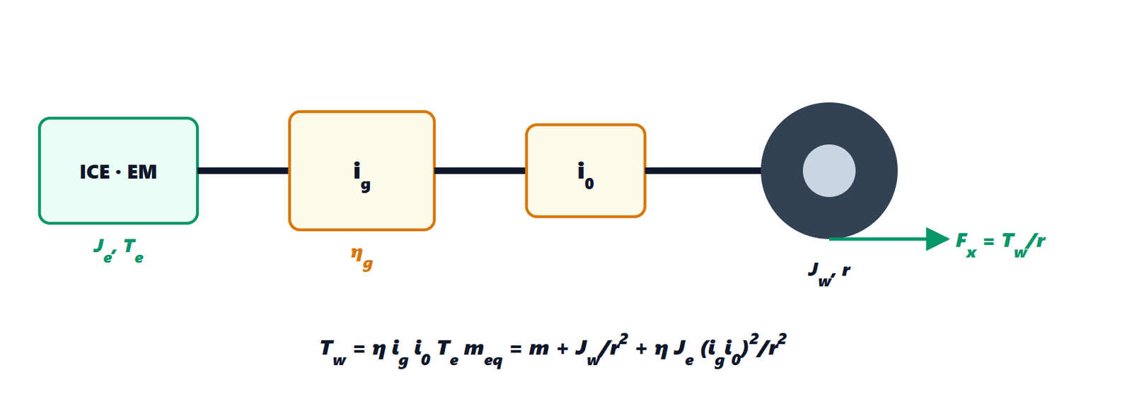
 , gearbox with ratio
 and efficiency
 , final drive
 , wheels of inertia
 and radius
 .
Accelerating the car means also accelerating everything that rotates. The equivalent mass comes from the kinetic energy: with the angular speed of the wheels  and of the engine
 ,

In a high gear  exceeds
 by a few percent (4% in our model), in first gear by as much as 30% (rotational dynamics explains why: the engine spins much faster than the wheels and the term grows with the square of the ratio).
The feedforward part: the inverse model
If we knew everything, the required torque would come from inverting the equation of motion:

This is the feedforward part: on its own it does almost all the work, with the estimates  and
 we will see shortly. What it does not know (the wind, model errors, the varying effectiveness of the brakes) is corrected by proportional-integral feedback on the acceleration error, with the acceleration derived from the wheel speeds:

The integral action needs a good anti-windup (see the PID controller): here there is no integration when the actuator of the active zone is at its limit, when a zone change is pending or has just happened, and in the intermediate zone. Without the second rule, during the waiting time before switching to the brakes the integral wound up and then made the car brake at −3.9 m/s² instead of the requested −3.0: we found it in the simulation and fixed it.
The three zones
The most delicate point is the split between engine and brakes. The natural boundary is the coast acceleration  : the one the car has with the pedal released and no brakes,

where  (−180 Nm at the wheels in our model) is the engine drag. Above the engine is enough; below it the brakes are needed.
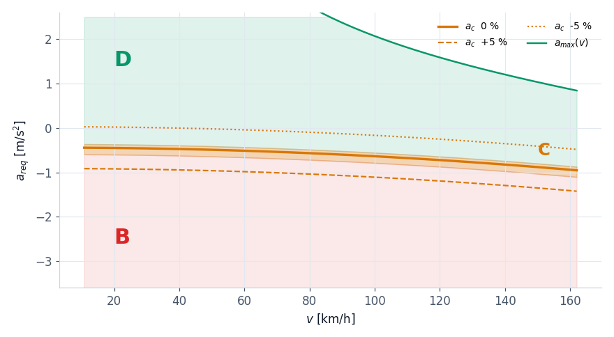 , B (brakes, red) below, C (coast, orange) in the band around . The curve depends a lot on the grade: at 100 km/h −0.64 m/s² on the flat, −1.11 on a 5% climb, −0.16 on a 5% descent. The green curve at the top is the power limit.
The hard case is precisely the intermediate band, because four problems add up there:
- small braking torques are imprecise: the first tens of Nm of pressure only overcome the piston return springs (in the model 25 Nm do not brake), pads away from the disc need 0.1 s to touch it, and light braking is noisy and wears the pads;
- the two actuators have different timing: the engine responds with a dead time and a time constant of 0.25 s, the brakes in 0.12 s;
- the request is noisy: it oscillates by a few hundredths of m/s² with the sensor measurements; with a sharp boundary it goes back and forth between engine and brakes;
- the boundary moves: it depends on the estimated speed, grade and mass.
The solutions, in the code:
- an acceptance band: in zone C the engine is released and the brakes do not work; the residual error (at most the width of the band, 0.08 m/s²) is accepted and the integral stops, so it does not wind up;
- minimum time in a zone (0.3 s) before changing it, except for real braking (more than 0.5 m/s² below ), which enters at once;
- minimum braking torque of 40 Nm when the brakes are active: either we brake effectively or we do not brake;
- step-free handover: entering the brakes, the engine does not go to zero all at once; the brakes give exactly the difference between the estimated engine torque (a model of its delay) and the total one, so the sum stays constant while the engine winds down;
- prefill: if in zone C the request falls quickly towards the brakes, 15 Nm bring the pads to the disc without braking.

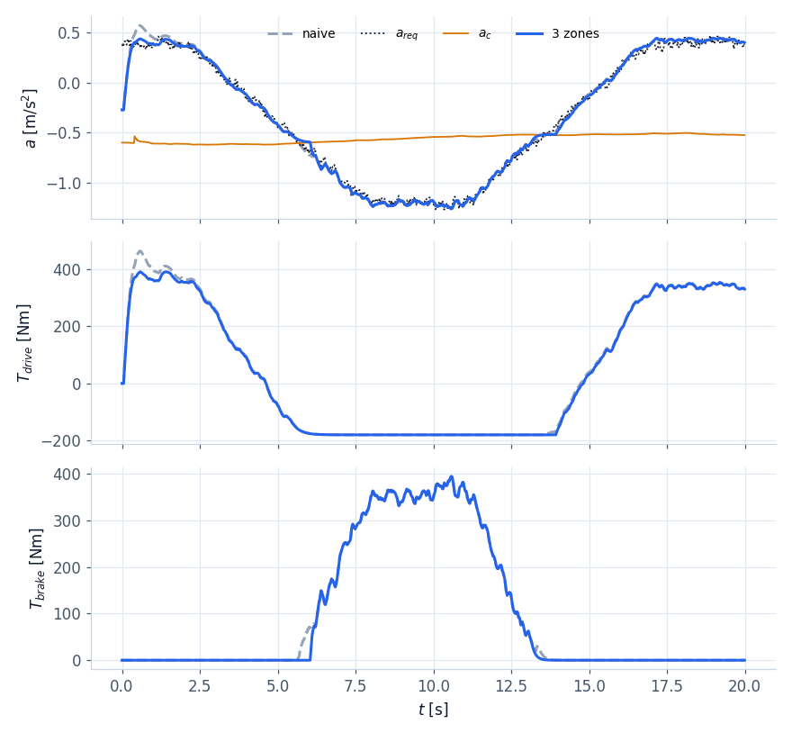
 , the minimum time
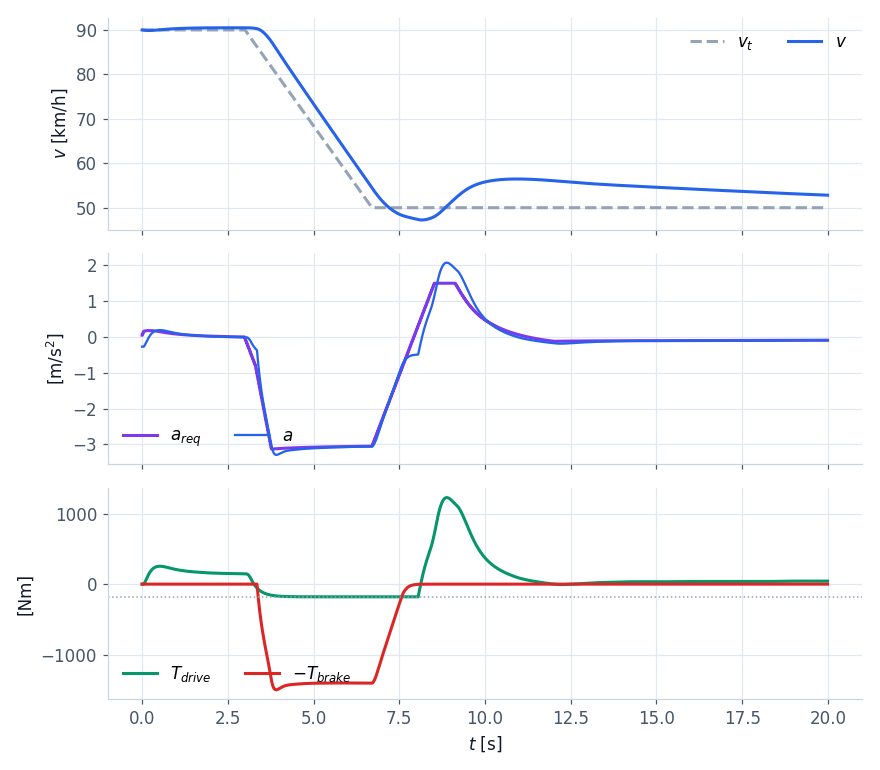
 , the immediate entry into the brakes for an urgent request. Each zone shows how the torques are split.
With an electric car zone C widens a lot: regenerative braking of the motor reaches −1.5 m/s² and beyond, and the split becomes one between regeneration (which recovers energy) and disc brakes (for hard braking or a full battery). The structure is the same, with the motor also working with negative torques.
Estimating grade and mass
The inverse model needs and . They come from signals every car already has.
Grade. The longitudinal accelerometer (in the inertial unit of the ESC) does not measure the acceleration of the car but the specific force: uphill, gravity “pulls” it backwards like a forward acceleration, and it measures  . The wheels instead measure only
 (differentiating the speed). Therefore
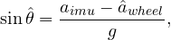
filtered with a 1 s time constant. A 0.03 m/s² error of the accelerometer (its offset) becomes a grade error of 0.3%: small, and feedback corrects it. With the vehicle stopped the formula gives the exact grade: it is needed to hold the car uphill.
Mass. While driving, without brakes, the equation of motion says

linear in the mass: it is a regression, and it is solved with least squares in recursive form (RLS), updating the estimate at every sample:

The forgetting factor  gives a memory of about 10 s. The estimate is updated only when the equation is reliable: no brakes (their torque is poorly known), speed above 18 km/h, acceleration of at least 0.3 m/s² (otherwise
 is small and the estimate picks up the noise).

The controller at work
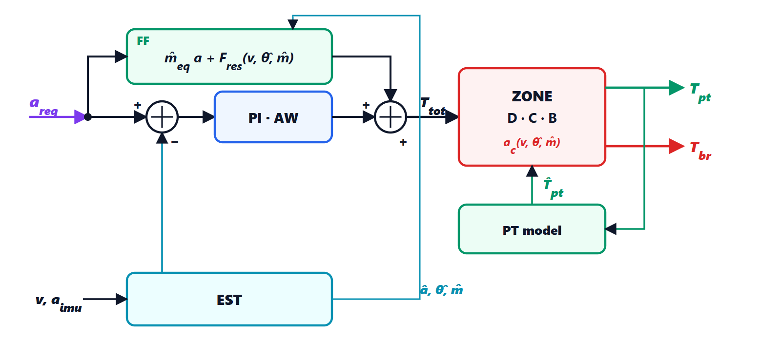 and the estimated acceleration, sum into
 , split into the zones based on , engine model giving the estimated torque
 for the handover to the brakes; the estimator (EST) derives
 , , from speed and accelerometer.
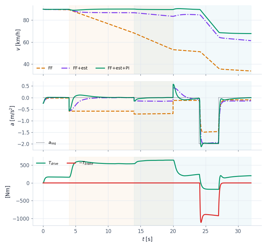
The toughest test bench: 90 km/h, and everything the controller does not know. A 350 kg payload, a 6% climb from 4 to 20 s, a 12 m/s headwind from 14 s, brakes 20% less effective (cold or worn pads), accelerometer offset; at the end a requested braking of 2 m/s².
Standing still, uphill
When the state machine is in STANDSTILL or WAIT (stop & go, lesson 5) the controller receives the hold command:
- hold: brakes at
 Nm, at least 800 Nm, and the integral reset. With the vehicle stopped the estimated grade is exact;
- drive-off without rolling back: below 0.5 m/s uphill the brakes hold the part of the weight that the engine does not give yet,
 , and they open as the engine torque grows. In the stop & go of lesson 5, on a 4% climb, the car does not roll back by a millimetre.
/* 2. zone around the coast acceleration, band + dwell time; urgent braking enters at once */
a_c = CoastAcceleration(p, v, c->sin_th, m);
want = a_req > a_c + c->b_hi ? Z_DRIVE : (a_req < a_c - c->b_lo ? Z_BRAKE : Z_COAST);
c->t_zone += ACC_DT;
urgent = want == Z_BRAKE && a_req < a_c - 0.5f;
if (want != c->zone && (c->t_zone >= c->t_dwell || urgent)) { c->zone = want; c->t_zone = 0.0f; }
sat = t_tot > t_hi || t_tot < t_lo || (c->zone == Z_DRIVE && t_tot < p->t_coast && e < 0.0f);
settling = want != c->zone || c->t_zone < c->t_dwell;
if (c->zone != Z_COAST && !sat && !settling) c->i_term += c->ki * e * ACC_DT;      /* anti-windup */
t_tot = clampf(t_tot, t_lo, t_hi);
/* 3. split: the brakes complement the ESTIMATED powertrain torque */
*t_pt = c->zone == Z_DRIVE ? t_tot : p->t_coast;
*t_br = c->zone == Z_BRAKE ? maxf(c->t_brake_min, c->t_pt_est - t_tot) : 0.0f;
We have all the pieces. In the last lesson we put them together and test them on a catalogue of scenarios with measurable criteria, in Python and in C.