ACC 7: integration, 14 test scenarios and Python and C code
The complete system, how an assistance function is tested, the scenario catalogue with measurable criteria, the bugs found, the C99 version with the same results and the code to download.
https://www.electronics-engineering.com/en/acc-integration-test-scenarios-python-c-code/
In the previous lessons we built every block of the ACC, from the radar measurement to the torque on the brakes. A block that works on its own, however, does not prove anything yet: real errors come from the interactions, when an overconfident tracker discards the camera, when an integral winds up during a zone change, when the state machine takes a slowdown for a stop. We found all of these precisely by putting the pieces together and testing them. In this lesson we look at the complete system, how it is tested, and the results: 14 scenarios in Python and 13 in C, all passed with measurable criteria.
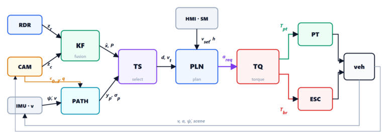
The complete system
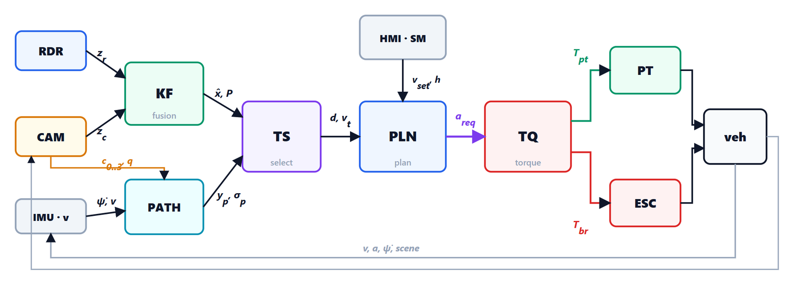
| Block | Lesson | Python (acc_sim.py) | C (acc.c) | Period |
|---|---|---|---|---|
| radar, camera | 2 | radar_measure, camera_measure | (in the sensor ECUs) | 50 / 66 ms |
| fusion | 3 | Tracker, Track | (Kalman: as in Python) | per measurement |
| path prediction | 4 | PathPredictor | PathPred_Run, PathPred_At | 20 ms |
| target selection | 4 | TargetSelector | TgtSel_Run | 20 ms |
| planner | 5 | Planner | Planner_Run | 20 ms |
| state machine | 1, 5 | AccStateMachine | AccSm_Run | 20 ms |
| torque control | 6 | TorqueController, Estimator | LongCtrl_Run | 20 ms (10 ms in the ESC) |
| vehicle (plant) | 6 | Vehicle | car_step in the test bench | 10 ms |
The main loop of the simulation has the same shape as an execution in the ECU: each block runs at its own rate and passes only its outputs to the next one.
for k in range(int(T / veh.dt)):                  # vehicle and sensors at 10 ms
    t = k * veh.dt
    tk.predict_to(t, veh.a)
    if k % 5 == 0:                                # radar, 20 Hz
        zs = [A.radar_to_cartesian(rp, m) for (x, y, v) in objs if (m := A.radar_measure(rp, rng, x - veh.x, y, v - veh.v))]
        if zs:
            tk.update(zs, A.H_RADAR, A.GATE_3D)
    if k % 7 == 3:                                # camera, about 15 Hz
        zs = [m for (x, y, v) in objs if (m := A.camera_measure(cp, rng, x - veh.x, y))]
        if zs:
            tk.update(zs, A.H_CAMERA, A.GATE_2D, init=False)
    if k % 2 == 0:                                # ADAS runnables, 20 ms
        tgt = ts.step(tk.tracks, pp.predict(veh.v, yaw_rate, lane), veh.v, 0.02, t)
        a_pl = pl.step(veh.v, (tgt.s[0], veh.v + tgt.s[1], 0.0) if tgt is not None else None)
        a_req = sm.step(driver, veh.v, a_pl, sensors_ok, t, pl.stop_request)
        t_pt, t_br, _ = tq.step(a_req, veh.v, veh.a_imu, hold=sm.hold)
    veh.step(t_pt, t_br, grade, wind)
How such a function is tested
An assistance function is tested at several levels, and the code of these lessons is ready for the first two:
- SIL (software in the loop): the real code, as it runs in the ECU, with a model of the vehicle and the sensors on a PC. This is what
test_scenarios.py(Python) andtest_acc.c(C) do; - HIL (hardware in the loop): the real ECU connected to a real-time simulator that generates the sensor and bus signals;
- track tests with moving targets (also the test procedures of ISO 15622 and Euro NCAP);
- road tests with thousands of recorded kilometres, replayed in simulation (re-simulation) with every new software version.
The rule that makes all of this useful: every scenario has a measurable criterion, decided before looking at the result. “The approach looks good” is not a test; “maximum deceleration below 2 m/s² and distance error below 5% after 60 s” is.
The scenario catalogue
| Scenario | Criterion | Result | Outcome |
|---|---|---|---|
| free cruise, from 100 to 120 km/h | speed error in the last 5 s < 1 km/h | 0.02 km/h | passed |
| approach from 130 to 80 km/h, 200 m | maximum deceleration < 2 m/s² | 0.75 m/s² | passed |
| approach from 130 to 80 km/h, 200 m | distance error after 60 s < 5% | 0.40% | passed |
| the target brakes at −4 m/s² to a stop | minimum distance > 2 m | 3.90 m | passed |
| cut-in at 50 m, 12 km/h slower (complete chain) | minimum distance > 15 m | 33.5 m | passed |
| cut-in at 50 m (complete chain) | maximum deceleration < 3.6 m/s² | 3.07 m/s² | passed |
| loss of radar measurements for 0.4 s | cycles without target = 0 | 0 | passed |
| car in the next lane at the entry of a curve, poor lines | time as a false target = 0 | 0 s | passed |
| stop & go on a 4% climb | stopping distance 4 ± 0.5 m | 3.93 m | passed |
| stop & go on a 4% climb | rollback < 0.1 km/h | 0.00 km/h | passed |
| stop & go on a 4% climb | WAIT, then RES, then ACTIVE | yes | passed |
| payload, 6% climb, headwind, weak brakes | speed error < 2 km/h | 0.36 km/h | passed |
| intermediate zone with a noisy request | changes between engine and brakes ≤ 4 | 4 | passed |
| sensor fault while braking | jerk of the request ≤ 2 m/s³ | 2.00 m/s³ | passed |
The criteria are not chosen at random: deceleration and jerk come from the standard (lesson 1), the distances from safety, the false positive and the loss of measurements from the situations that ruin the driver’s trust, the zone changes from comfort.
Almost every row of this table had, during development, a wrong first result, and each one taught something:
- fusion worse than the camera alone (process noise too small, lesson 3);
- the “elastic” approach braking more than the normal one (the mild phase could brake more than necessary, lesson 5);
- stopping at 15 m instead of 4 (the state machine took a slowdown for a stop, and the planner copied the target’s braking instead of aiming at its stopping point, lesson 5);
- braking at −3.9 m/s² instead of −3 (integral wound up during the waiting time of the zone change, lesson 6);
- rolling back uphill (the brakes opened in the coast zone at almost zero speed, lesson 6);
- the short time gap making the string unstable (fixed gains, lesson 5).
This is why automatic tests matter more than any review by eye.
The same chain in C
The C99 version (acc.h, acc.c) is written as AUTOSAR components: every component has an initialisation function and a runnable with explicit inputs and outputs, no dynamic memory, no recursion, only float. The test bench test_acc.c contains a vehicle model (engine with dead time and delay, brakes with springs and pad clearance, static friction at standstill) and 13 scenarios:
Approach 130 -> 80 km/h                  peak deceleration [m/s2]            0.74  PASS
Approach 130 -> 80 km/h                  gap error after 60 s [%]            0.52  PASS
Stop & go, 4 % climb                     stops                               2.00  PASS
Stop & go, 4 % climb                     1st stop distance (d0 = 4) [m]      3.94  PASS
Stop & go, 4 % climb                     2nd stop distance (d0 = 4) [m]      3.95  PASS
Stop & go, 4 % climb                     rollback speed [km/h]              -0.00  PASS
Stop & go, 4 % climb                     WAIT then RES -> ACTIVE             1.00  PASS
Cut-in, lateral speed 1 m/s              locked at t [s] (python 3.9)        3.90  PASS
Next-lane car at 95 m, no lines          time locked [s]                     0.00  PASS
Coast zone, noisy request                zone changes (4 needed)             4.00  PASS
Coast zone, noisy request                max |a - a_req| [m/s2]              0.09  PASS
Payload 350 kg + 6 % climb               max speed error [km/h]              0.36  PASS
Sensor fault while braking               jerk of the request [m/s3]          2.00  PASS

13/13 PASS
It compiles without a single warning with gcc -std=c99 -O2 -Wall -Wextra -Wpedantic -o test_acc acc.c test_acc.c -lm. The results match the Python ones (stops at 3.94 and 3.95 m against 3.93 and 3.94, cut-in locked at 3.90 s against 3.92, speed error 0.36 km/h in both): two independent implementations of the same algorithm giving the same numbers are strong evidence that both do what the theory says.
The parameters
| Parameter | Value | Where | Why |
|---|---|---|---|
| time gap | 1.0 / 1.4 / 1.8 / 2.2 s | state machine | four settings, the standard asks for ≥ 0.8 and one between 1.5 and 2.2 |
 | 4 m | planner | distance at standstill |
 ,  ,  | 0.15, 0.6 (or more), 0.3 | planner | damping > 1, string stability  |
elasticity  | 0.25 h v, at most 12 m | planner | softer braking in the approach |
| preboost | 0.9 s, +0.6 m/s², 4 s | planner | smoother overtaking, never below 0.9 s |
 ,  | 0.60, 0.35 | selection | hysteresis |
 | 0.3 + 0.25  s | selection | longer confirmation if the path is uncertain |
 | 0.6 s | selection | short loss of measurements |
 ,  | 2.0, 1.5 m/s² | fusion | real manoeuvres (lane change) |
| zone C band | ± 0.08 m/s² | torque | about the minimum useful braking torque |
| minimum time in a zone | 0.3 s | torque | no engine/brake oscillations |
 ,  | 0.6, 1.2 | torque | correction of model errors |
Where this subject sits
The seven lessons are in the Automotive subject, with their syllabus; they use tools from other subjects, which they refer to where needed:
- Automatic control: stability, second-order response, PID and anti-windup (lessons 5 and 6);
- Digital control: Kalman filter, observers, discretisation, computation delay, optimal and predictive control (lessons 1, 3, 5);
- Communications and Electromagnetic fields: the FMCW radar (lesson 2);
- Physics 1: dynamics, inclined plane, rotation (lesson 6);
- Numerical methods and Mathematical methods: least squares, Gaussian and probability (lessons 3, 4, 6).
Where to go from here
The code is a real starting point, but a series ACC still requires:
- calibration on the vehicle: the parameters of the engine, the brakes and the comfort tables are measured on the car, not invented;
- several motion models in the tracker (IMM) and probabilistic association in dense traffic;
- the next lane for the preboost, from the corner radars, and the prediction of the trajectories of other vehicles;
- functional safety: hazard analysis (ISO 26262), independent monitors of the requests, fault injection tests;
- homologation and Euro NCAP tests, which use scenarios very similar to those in the table.
Download the complete code (zip, 42 kB): acc_sim.py, make_plots.py, test_scenarios.py, acc.h, acc.c, test_acc.c and instructions. It needs Python 3.8 or newer with numpy (matplotlib for the charts) and a C99 compiler.
The code is meant to be read, changed and run again: change a parameter, rerun the tests and see which criterion stops being met. It is the quickest way to understand why every detail of the previous lessons is there.