ACC 3: radar and camera fusion with the Kalman filter
Centralised and track-to-track fusion, relative motion model, Kalman gain proved, why two sensors beat one, gating, association, track management and a tuning mistake.
https://www.electronics-engineering.com/en/acc-radar-camera-fusion-kalman-filter-association-tracks/
Radar and camera send, each at its own rate, lists of measurements that are noisy, sometimes missing, sometimes false. Fusion turns them into a list of tracked objects: for each one an estimate of position and speed with its uncertainty, updated every cycle. The tool is the Kalman filter, which we introduced in the lesson on the Kalman filter and met again among the discrete observers; here we apply it to several sensors, add the association of measurements to objects and track management, and look at a tuning mistake that makes fusion worse than a single sensor.
Two architectures
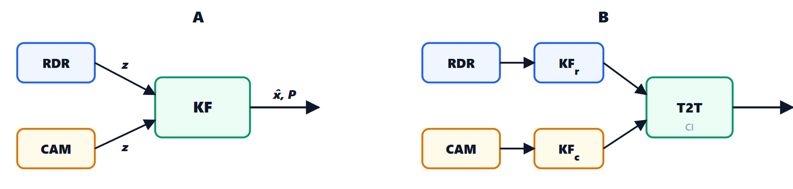
- centralised (A): the most precise, because the filter uses every measurement with its true uncertainty; it needs raw or nearly raw, time-stamped measurements;
- track-to-track (B): each sensor ECU already does its own tracking (common with sensors from different suppliers) and the ADAS ECU fuses the tracks. Two tracks of the same object have correlated errors (they share the same motion model), and treating them as independent would make the estimate overconfident. Covariance intersection is safe even without knowing the correlation:
 ,
 , with
 chosen to minimise the trace of
 .
In the code we use centralised fusion.
The model of relative motion
The state of each object is relative to our car:  . Longitudinally the relative acceleration is
 : the target’s
 is unknown and we treat it as noise, our own
 is known and we use it as an input. Integrating over a step
 with constant acceleration (see the kinematics of linear motion):

and the same laterally, without input. In matrix form  with

 and
 are the standard deviations of the accelerations the model does not know: how hard the target can brake or accelerate, how quickly it can move sideways. Their value matters a lot, as we will see.
The Kalman filter
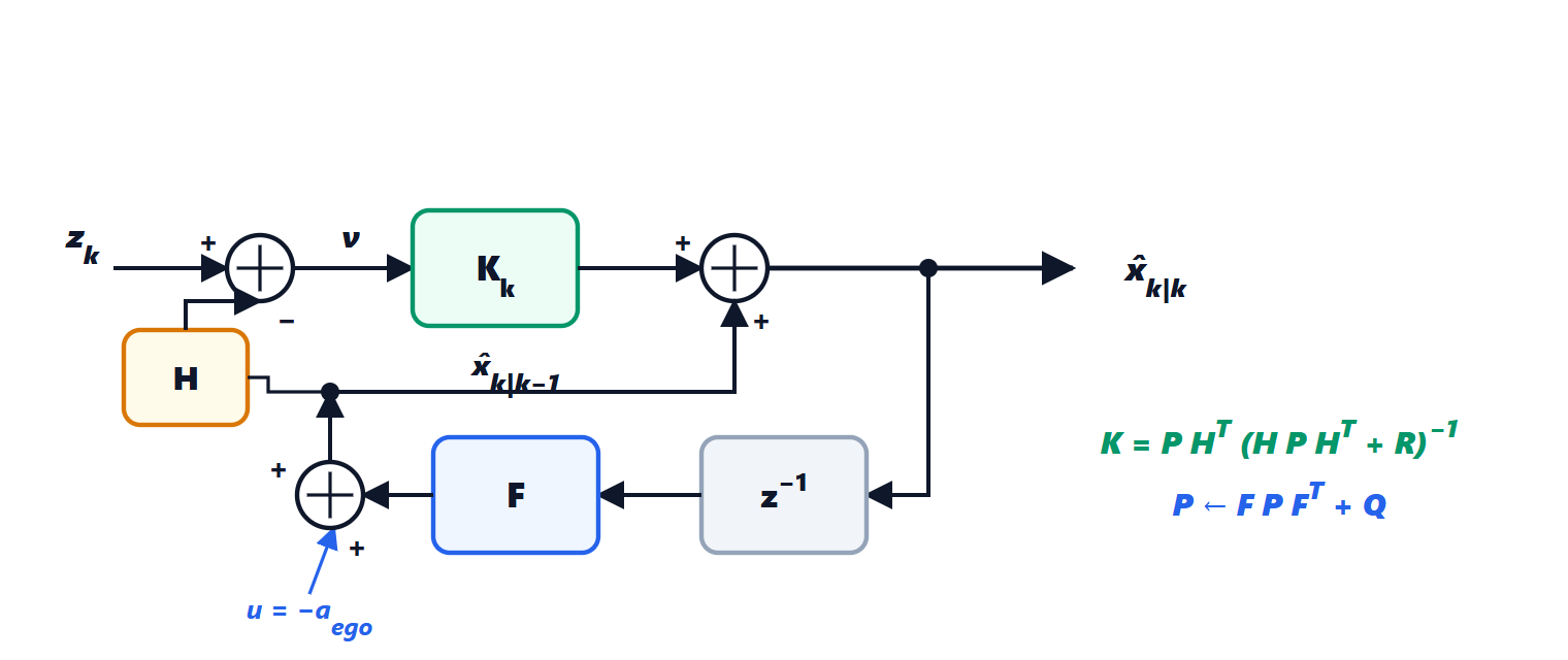
 and the model
 (with the input
 ) and becomes the prediction
 ; the measurement
 minus the predicted measurement
 is the innovation
 , which multiplied by the gain
 corrects the prediction.
For every measurement the filter takes two steps:
- prediction up to the time of the measurement:
 ,
 ;
- update: innovation
 , its covariance
 , gain
 , then
 ,
 .
Why that gain. After the correction the error is  , with
 the prediction error and
 the measurement noise, independent. Its covariance is

(this is the Joseph form, which we also use in the code because it stays symmetric and positive with floating point numbers). We look for the  that minimises the sum of the variances, the trace of
 . Expanding and differentiating with respect to , with
 for symmetric
 :

Why two sensors are better than one
The simplest case says it all. Two independent estimates of the same quantity,  with variance
 and
 with
 : their weighted mean
 has variance
 , minimum for
 . Substituting:
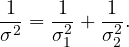
Information (the inverse of the variance) adds up: the fused estimate is always better than the better of the two. And this is exactly what the Kalman filter does, component by component: for the distance it weights mostly the radar, for the lateral position mostly the camera (the formulas of the Gaussian give the same result with Bayes’ theorem).
The measurements of the two sensors
The camera gives  with covariance
 derived in lesson 2:
 takes the first and third components of the state. The radar measures in polar coordinates
 ; to use a linear filter the measurement is converted to Cartesian coordinates,
 ,
 , and the covariance is propagated with the Jacobian matrix:

For a target ahead ( ) the error ellipse is narrow in
 (
 ) and wide in
 (
 ). The radial speed
 is the third measurement. The sensors are not synchronised (radar at 20 Hz, camera at 15 Hz): the filter predicts each object up to the time of the measurement and uses it right away, in time order.
Associating measurements to objects
Before updating we have to know which measurement belongs to which object.
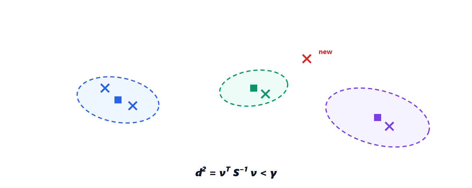
- validation gate (gating): the Mahalanobis distance
 of a correct measurement follows a
 distribution with as many degrees of freedom as the components of the measurement. We accept the measurement if
 , with
 (2 degrees, camera) or 11.34 (3 degrees, radar) for 99%. Unlike the Euclidean distance, the gate widens where the track is uncertain;
- global association (Global Nearest Neighbour): among all possible assignments (each track at most one measurement, each measurement at most one track) we pick the one with the most pairs and the smallest sum of distances. With few objects all can be tried; with many the Hungarian algorithm does it in
 . In dense traffic or with many false echoes probabilistic methods are used (JPDA, MHT), seen in the lesson on radar tracking.
Managing the tracks
A measurement that is not associated starts a tentative track; it becomes confirmed when it has been associated in at least 3 of the last 5 cycles (M-of-N logic), and it is deleted after 6 cycles without measurements. Only confirmed tracks go to target selection: an isolated echo (a reflection, an insect on the radome) never reaches the planner.
def update(self, z, R, H):
    y = z - H @ self.s                   # innovation
    S = H @ self.P @ H.T + R             # innovation covariance
    K = self.P @ H.T @ np.linalg.inv(S)  # Kalman gain
    self.s = self.s + K @ y
    I_KH = np.eye(4) - K @ H
    self.P = I_KH @ self.P @ I_KH.T + K @ R @ K.T   # Joseph form
    return y, S
A mistake that makes fusion worse than one sensor
In the simulation a car ahead, from 30 to 110 m, changes lane at some point. With the first tuning,  m/s², the result was paradoxical: root mean square lateral error 0.32 m fusing radar and camera, 0.11 m with the camera alone. Fusion was worse than the better sensor.
The cause: with many measurements and a small the filter became overconfident,  cm. During the lane change (a true lateral acceleration of about 1 m/s²) the camera measurements, which were correct, fell outside the validation gate of such a self-assured filter and were discarded: 36 out of 222. Only the radar was left, imprecise sideways, and the track followed the manoeuvre late.
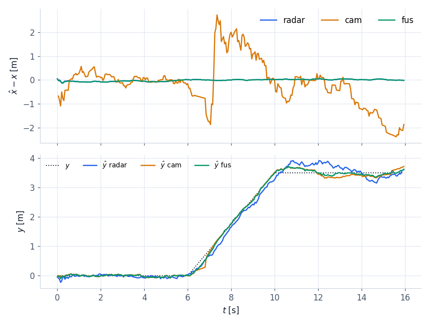
 m/s²: top, distance error (radar and fusion 0.03 m, camera 1.1 m); bottom, the estimated lateral position during the lane change between 6 and 10 s. Fusion (green) follows the manoeuvre better than either sensor: error 0.08 m against 0.19 m for the radar and 0.11 m for the camera.
With m/s², a value that covers a real manoeuvre, fusion does its job again: 0.03 m in distance (like the radar) and 0.08 m sideways (better than the camera). The general lesson: process noise is not a smoothing parameter, it is a statement about how much objects can move; if it is too small the filter throws reality away. Series systems often use several models together (IMM, Interacting Multiple Models): a constant velocity one for quiet stretches and a manoeuvre one, weighted according to which explains the measurements better.
The tracker now gives a list of objects with state and covariance. Which one should we follow? That is the problem of the next lesson, and it is where an ACC earns the driver’s trust or loses it.