Radar tracking: measurement accuracy and the Cramér-Rao bound, α-β and Kalman filters, IMM and association

Resolution and accuracy, the Cramér-Rao bound checked with a simulation, the classic tracking radar and monopulse, α-β and Kalman filters with the trade-off between noise and responsiveness, the IMM filter, gating and GNN, JPDA and MHT association.

ielettronica 12 November 2018 Updated 25 October 2026 11 min read 0 comments

Finding a target is not enough: an air traffic control radar, a naval radar or a car radar must follow it over time, estimate its position and velocity better than any single measurement says, predict where it will be and recognise when it is manoeuvring. This is tracking. This lesson starts from the accuracy with which the radar measures range, angle and velocity (parameter estimation, with the Cramér-Rao bound), goes through the classic tracking radar, which follows a single target with the antenna, and arrives at the filters used today in every system: the α-β filter, the Kalman filter, the association between measurements and tracks when there are many targets, and multiple model filters for manoeuvres. A simulation shows the fundamental trade-off between noise and responsiveness.

The idea in simple words

Following a target with a radar is like following a ball with your eyes during a match watched through a dirty window: sometimes you see it clearly, sometimes it appears displaced, but your brain does not jump after every image; it imagines where the ball should be (because it knows the ball moves with a certain speed) and corrects this idea a little with what it sees. If the ball suddenly changes direction, for a moment the brain “lags behind”, then catches up.

A tracking filter does the same with formulas: it predicts where the target will be, measures, and corrects the prediction with part of the difference. How much to correct is the key choice: correcting little gives a smooth track that is slow to follow manoeuvres, correcting a lot gives a responsive but jittery track. The Kalman filter computes the best correction knowing how accurate the measurements are (the first part of the lesson) and how unpredictable the target is.

A bit of history

Radar is associated with microwaves, but the first echo-ranging systems were the short-wave (HF) soundings used in the 1920s by Breit and Tuve to measure the height of the ionosphere. The first operational radars, the Chain Home network built by the British at the end of the 1930s to detect enemy aircraft and later V-2 missiles, also worked in the upper part of the short-wave band (wavelengths of about ten metres), because the technology of the time did not allow higher frequencies: in a sense they were the ancestors of over-the-horizon (OTH) radars. The cavity magnetron (1940) brought radar to microwaves, with small antennas and narrow beams, and made fire-control and tracking radars possible.

The classic tracking radar

A tracking radar keeps the target at the centre of the beam with servomechanisms:

in range, with a range gate split into two halves, early and late: if the echo falls more in the late half, the gate moves forward (early-late gate);
in angle, with conical scan (the beam rotates around the axis and the echo is amplitude-modulated if the target is off centre) or, much better, with the monopulse of the lesson on phased arrays, which measures the error with a single pulse and is insensitive to amplitude fluctuations (a jammer that modulates its power at the scan frequency easily deceives conical scan).

Modern array radars instead track many targets “time-shared”: the beam jumps from one target to another, and continuity is provided by the tracking filter, which is the subject of the rest of the lesson. The same holds for surveillance radars (one measurement per antenna turn) and car radars (one measurement about every 50 ms).

Measurement accuracy: parameter estimation

Before filtering the measurements one must know how accurate they are. Do not confuse resolution and accuracy: resolution ( $c/2B$ in range, the beamwidth in angle, $\lambda/2T_{obs}$ in velocity) says how far apart two targets must be to be seen as separate; accuracy says with what error the position of one isolated target is measured. With a good signal-to-noise ratio accuracy is much better than resolution, because the centre of a wide peak can be located with a small error, as one reads a thermometer between two marks.

The Cramér-Rao bound. Statistics gives a lower bound on the error of any unbiased estimator: for the delay $\tau$ of an echo in white noise,

$\sigma_\tau \ge \frac{1}{\beta\sqrt{2\,SNR}},\qquad \beta^2 = \frac{\int(2\pi f)^2|S(f)|^2df}{\int|S(f)|^2df}$

where $SNR$ is the peak signal-to-noise ratio after the matched filter and $\beta$ the effective (rms) bandwidth of the signal. For a flat spectrum $B$ wide, $\beta = 2\pi B/\sqrt{12} = 1.81\,B$ , and in range $\sigma_R = \frac{c}{2}\sigma_\tau = 0.55\,\frac{c/2B}{\sqrt{2\,SNR}}$ . The textbook rule of thumb, 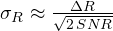$\sigma_R \approx \frac{\Delta R}{\sqrt{2\,SNR}}$ , has the same form with a constant that depends on the spectrum. The message is clear: accuracy improves as the square root of the signal-to-noise ratio and in proportion to bandwidth.

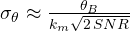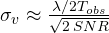Similarly, for angle (with monopulse) $\sigma_\theta \approx \frac{\theta_B}{k_m\sqrt{2\,SNR}}$ , with $k_m \approx 1.6$ the monopulse slope; for velocity $\sigma_v \approx \frac{\lambda/2T_{obs}}{\sqrt{2\,SNR}}$ .

Simulation. An echo with 1 MHz of bandwidth (150 m resolution), estimated with the matched filter and a fine peak search, 1000 trials for each level:

SNR	simulated error	Cramér-Rao bound	rule of thumb
30 dB	1.8 m	1.8 m	3.4 m
20 dB	5.6 m	5.8 m	10.6 m
10 dB	19.8 m (plus 7.8 % of gross errors)	18.2 m	33.5 m

At high SNR the estimator reaches the theoretical bound (the small difference below the bound at 20 dB is due to the finite number of trials, which gives an uncertainty of a few per cent on the estimated standard deviation): at 20 dB the error is 5.6 m, almost thirty times smaller than the resolution. At low SNR the threshold effect appears: sometimes the noise makes a sidelobe win and the error becomes gross (hundreds of metres). For angle, with a 2° beam and 20 dB, $\sigma_\theta = 0.088°$ : at 50 km that is 77 m of cross-range error, much more than the 6 m in range. For velocity, with 64 ms of observation in X band, the resolution is 0.23 m/s and the accuracy 1.7 cm/s. These are the values of $\sigma$ to put into the measurement model of the Kalman filter, and they explain why the uncertainty of a track is an ellipse elongated in the cross-range direction.

import numpy as np

# range measurement accuracy: simulation against the Cramér-Rao bound
c, B = 299792458.0, 1e6                                # 1 MHz bandwidth: resolution c/2B = 150 m
N, fs = 256, 4e6                                       # samples in the frequency domain, sampling rate
f = np.fft.fftfreq(N, 1 / fs)
S = (np.abs(f) <= B / 2).astype(float)                 # flat spectrum B wide
E = np.sum(S ** 2)
rng = np.random.default_rng(0)
true_delay = 10.3 / fs                                 # echo at 10.3 samples: not on a sample
for snr_dB in (10, 20, 30):
    snr = 10 ** (snr_dB / 10)                          # peak signal-to-noise ratio after the matched filter
    sig_n = np.sqrt(E / snr)                           # noise per complex component in frequency
    errors = []
    grid = np.linspace(-0.6, 0.6, 601) / fs            # fine search around the coarse peak
    for _ in range(1000):
        R = S * np.exp(-2j * np.pi * f * true_delay) + sig_n * (rng.normal(size=N) + 1j * rng.normal(size=N)) / np.sqrt(2)
        Y = R * S                                      # matched filter in the frequency domain
        t0 = np.argmax(np.abs(np.fft.ifft(Y))) / fs
        tt = t0 + grid
        out = np.abs(np.exp(2j * np.pi * np.outer(tt, f)) @ Y)
        errors.append(tt[np.argmax(out)] - true_delay)
    err = np.array(errors) * c / 2
    gross = np.abs(err) > c / (2 * B)                  # the peak landed on a wrong lobe
    beta = np.sqrt(np.sum((2 * np.pi * f) ** 2 * S ** 2) / E)     # effective (rms) bandwidth
    crb = c / 2 / (beta * np.sqrt(2 * snr))
    print(f"SNR {snr_dB} dB: simulated error {np.std(err[~gross]):5.1f} m ({gross.mean() * 100:.1f} % gross errors), "
          f"Cramér-Rao {crb:5.1f} m, rule of thumb c/2B/sqrt(2 SNR) {c / (2 * B) / np.sqrt(2 * snr):5.1f} m")

# angle and velocity accuracy with the approximate formulas
snr = 100.0
print(f"angle: 2 degree beam, km = 1.6, SNR 20 dB: {2 / (1.6 * np.sqrt(2 * snr)):.3f} degrees, that is {50e3 * np.radians(2 / (1.6 * np.sqrt(2 * snr))):.0f} m at 50 km")
lam, Tobs = 0.03, 64e-3
print(f"velocity: resolution {lam / (2 * Tobs):.3f} m/s, accuracy with SNR 20 dB {lam / (2 * Tobs) / np.sqrt(2 * snr):.4f} m/s")

The α-β filter

The target moves at roughly constant velocity; at every measurement $z_k$ (with period $T$ ) the filter predicts where it should be and then corrects the prediction with a fraction of the error (the innovation $r_k$ ):

$\hat x_k^- = \hat x_{k-1} + T\hat v_{k-1},\qquad r_k = z_k - \hat x_k^-,\qquad \hat x_k = \hat x_k^- + \alpha r_k,\qquad \hat v_k = \hat v_{k-1} + \frac{\beta}{T}r_k$

With small $\alpha$ and $\beta$ the filter “trusts” the prediction and averages many measurements (little noise, but slow response to a manoeuvre); with large values it follows the measurements (responsive, but noisy). A classic choice linking the two parameters is that of Benedict and Bordner, $\beta = \frac{\alpha^2}{2 - \alpha}$ .

The Kalman filter

The Kalman filter (1960) generalises the α-β: it describes the target with a state model $\mathbf x_k = F\mathbf x_{k-1} + \mathbf w_k$ (for example position and velocity, with a random acceleration $\mathbf w$ of covariance $Q$ ) and the measurement with $z_k = H\mathbf x_k + n_k$ (noise of variance $R$ ), and computes at every step the optimum gain from the uncertainty $P$ of the estimate:

$\text{prediction:}\quad \hat{\mathbf x}^- = F\hat{\mathbf x},\quad P^- = FPF^T + Q$

$\text{correction:}\quad K = P^-H^T(HP^-H^T + R)^{-1},\quad \hat{\mathbf x} = \hat{\mathbf x}^- + K(z - H\hat{\mathbf x}^-),\quad P = (I - KH)P^-$

For a linear system with Gaussian noises it is the minimum-variance estimator (its derivation is in the article on the Kalman filter linked to this lesson). After a few steps $P$ and $K$ settle: the steady-state Kalman filter is an α-β filter, with $\alpha$ and $\beta$ set by the ratio between the process noise $Q$ and the measurement noise $R$ . The advantage of the Kalman filter is that it works well also in the initial transient, with variable measurement periods, with measurements of different kinds (range, angles, Doppler) and in several dimensions.

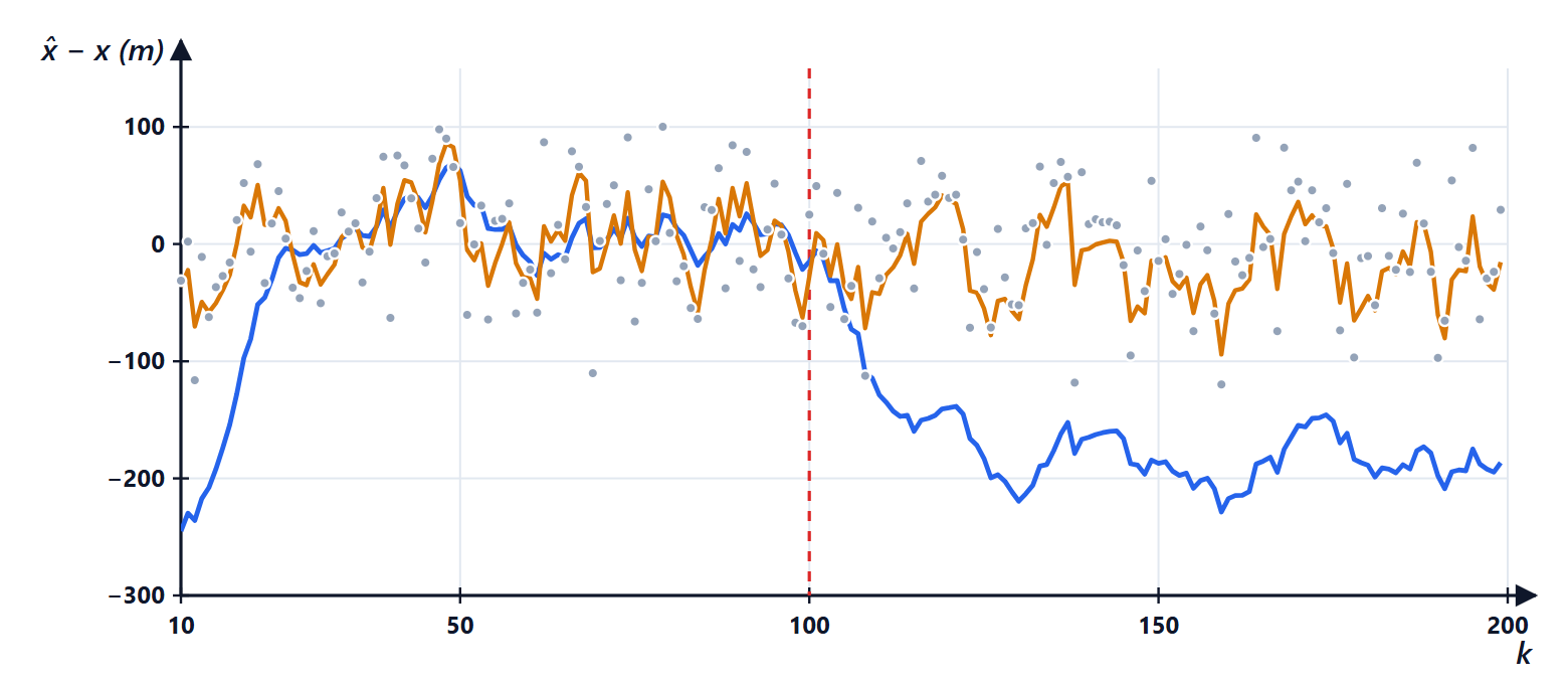
Tracking a target that accelerates halfway — The estimation error over time: the slow filter, blue, has little noise in the uniform stretch but builds up a large lag when the target accelerates, after second 100; the fast filter, orange, is noisier but follows the manoeuvre. The grey dots are the errors of the individual measurements.

The simulation: noise versus responsiveness

A target at 100 m/s, measured once per second with a 50 m error, which after 100 seconds starts accelerating at 5 m/s². Rms error of the estimates (the measurements alone have 48 m):

filter	uniform motion	manoeuvring
α-β with α = 0.2	25 m	181 m
α-β with α = 0.5	33 m	37 m
Kalman with q = 0.1	16 m	696 m
Kalman with q = 10	26 m	73 m

No fixed filter works well in both situations: the one that filters uniform motion well loses the target in a manoeuvre, the one ready for manoeuvres is noisy. The Kalman filter with $q = 10$ reaches steady state with $\alpha = 0.299$ and $\beta = 0.053$ , practically the Benedict-Bordner pair ( $0.3^2/1.7 = 0.053$ ).

The solution: several models together. The IMM filter (interacting multiple model) runs several Kalman filters in parallel, for example one for uniform motion and one for manoeuvres, and combines them weighted by the probability that each model is the right one, computed from the innovations. When the target manoeuvres, the innovation of the “uniform” filter grows, its weight drops and the “manoeuvre” filter prevails. It is the standard in air surveillance systems and automotive radars.

Many targets: initiation and association

With many targets and false alarms one must decide which measurement belongs to which track:

gating: only measurements close enough to the prediction are considered for a track, measuring the distance with the uncertainty (Mahalanobis distance $r^TS^{-1}r$ , compared with a threshold of the chi-square distribution);
association: with the global nearest neighbour rule (GNN, optimal assignment with the Hungarian algorithm), or with probabilistic methods that weight all compatible measurements (JPDA), or keeping several alternative hypotheses until the data resolve them (MHT);
initiation and deletion: a new track is born from unassociated measurements and is confirmed if it appears again, for example, in 3 scans out of 5 (M-of-N logic); a track without measurements for too many scans is deleted.

The same tools serve to assemble objects from the points of a car radar, in the dedicated lesson.

Summary

Resolution and accuracy are different things: accuracy improves as the square root of the signal-to-noise ratio and reaches the Cramér-Rao bound.
In angle the cross-range error grows with range: the uncertainty of a track is an elongated ellipse.
The α-β filter predicts and corrects with fixed gains; the Kalman filter computes the optimum gains, and in steady state coincides with an α-β.
No fixed filter works both in uniform motion and in manoeuvres: the IMM combines several models.
With many targets, gating, association (GNN, JPDA, MHT) and track confirmation logic are needed.

The code

import numpy as np

rng = np.random.default_rng(0)
T, steps, sigma = 1.0, 200, 50.0                     # one measurement per second, 50 m measurement error
k = np.arange(steps)
true = 1000 + 100 * k * T + 0.5 * 5.0 * (np.maximum(k - 100, 0) * T) ** 2   # 100 m/s, then accelerates at 5 m/s^2
z = true + rng.normal(0, sigma, steps)               # range measurements

def alpha_beta(alpha):
    beta = alpha ** 2 / (2 - alpha)                  # Benedict-Bordner choice
    x, v, estimates = z[0], 0.0, []
    for zk in z:
        xp = x + v * T                               # prediction
        r = zk - xp                                  # innovation: measurement minus prediction
        x, v = xp + alpha * r, v + beta / T * r      # correction
        estimates.append(x)
    return np.array(estimates), beta

def kalman(q):
    F = np.array([[1, T], [0, 1]]); H = np.array([[1.0, 0.0]])
    Q = q * np.array([[T ** 4 / 4, T ** 3 / 2], [T ** 3 / 2, T ** 2]])   # random acceleration of variance q
    R = np.array([[sigma ** 2]])
    x, P, estimates, gains = np.array([z[0], 0.0]), np.diag([sigma ** 2, 1e4]), [], []
    for zk in z:
        x, P = F @ x, F @ P @ F.T + Q                # prediction
        S = H @ P @ H.T + R
        K = P @ H.T / S                              # Kalman gain
        x = x + (K * (zk - H @ x)).ravel()
        P = (np.eye(2) - K @ H) @ P
        estimates.append(x[0]); gains.append(K.ravel())
    return np.array(estimates), gains[-1]

def rms(s, a, b):
    return np.sqrt(np.mean((s - true)[a:b] ** 2))

for alpha in (0.2, 0.5):
    s, beta = alpha_beta(alpha)
    print(f"alpha-beta alpha = {alpha}, beta = {beta:.3f}: error {rms(s, 20, 100):5.1f} m in uniform motion, {rms(s, 110, 200):6.1f} m manoeuvring")
for q in (0.1, 10.0):
    s, K = kalman(q)
    print(f"Kalman q = {q:4}: error {rms(s, 20, 100):5.1f} m and {rms(s, 110, 200):6.1f} m; steady-state gains alpha = {K[0]:.3f}, beta = {K[1] * T:.3f}")
print(f"error of the measurements alone: {np.sqrt(np.mean((z - true) ** 2)):.1f} m")

Running the first program prints the rows of the accuracy table and the angle and velocity accuracies (0.088°, 77 m, 0.234 m/s and 0.0166 m/s). The second prints the rows of the filter table: 25.2 and 180.8 m, 33.0 and 36.7 m, 16.3 and 695.6 m with gains 0.106 and 0.006, 25.5 and 73.1 m with gains 0.299 and 0.053, and 48.1 m for the measurements alone.

0 Comments

Oldest

Newest Most Voted

Cookie	Duration	Description
cookielawinfo-checkbox-analytics	11 months	This cookie is set by GDPR Cookie Consent plugin. The cookie is used to store the user consent for the cookies in the category "Analytics".
cookielawinfo-checkbox-functional	11 months	The cookie is set by GDPR cookie consent to record the user consent for the cookies in the category "Functional".
cookielawinfo-checkbox-necessary	11 months	This cookie is set by GDPR Cookie Consent plugin. The cookies is used to store the user consent for the cookies in the category "Necessary".
cookielawinfo-checkbox-others	11 months	This cookie is set by GDPR Cookie Consent plugin. The cookie is used to store the user consent for the cookies in the category "Other.
cookielawinfo-checkbox-performance	11 months	This cookie is set by GDPR Cookie Consent plugin. The cookie is used to store the user consent for the cookies in the category "Performance".
viewed_cookie_policy	11 months	The cookie is set by the GDPR Cookie Consent plugin and is used to store whether or not user has consented to the use of cookies. It does not store any personal data.

The idea in simple words

A bit of history

The classic tracking radar

Measurement accuracy: parameter estimation

The α-β filter

The Kalman filter

The simulation: noise versus responsiveness

Many targets: initiation and association

Summary

The code

Related articles

From imitation to reinforcement learning: how Chinese driving systems are trained

China’s new rules for assisted and automated driving (GB 47955 and GB 44721)

The chips and sensors behind China’s assisted driving

Navigate on Autopilot in China: how city NOA became a mass-market feature

Robotaxis in China in 2026: Baidu Apollo Go, Pony.ai and WeRide

SAR, weather radars and military radars: synthetic aperture, reflectivity, jamming and burn-through