Probability for signals: Bayes, random variables and the Gaussian
Conditional probability, Bayes' theorem with proof and an example, mean and variance, the Gaussian distribution and the Q function, sums of independent variables, the central limit theorem.
The noise of an amplifier, the bits sent over a channel, the arrival times of packets in a network cannot be predicted individually, but they have precise statistical regularities. Describing them requires probability theory. In this lesson we review the essential tools for signals: conditional probability and Bayes’ theorem, random variables, mean and variance, the Gaussian distribution and the central limit theorem.
Probability and conditional probability
A probability assigns each event a number between 0 and 1, with  and
 for mutually exclusive events. The conditional probability of
 given that
 has occurred is
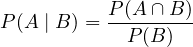
Two events are independent if  , that is if knowing that one has occurred does not change the probability of the other.
Bayes’ theorem
Theorem. If  are mutually exclusive events covering all possible cases,

Proof. From the definition,  , so
 . Since the
 cover all cases without overlapping,
 (total probability). ∎
Bayes “reverses” the conditioning: from the observed effect it goes back to the most probable cause. It is the logic of every receiver: having observed a signal, which symbol was sent?
Example. A diagnostic test detects a disease in 99% of sick people and gives a false positive in 5% of healthy people; the disease affects 1% of the population. With a positive test, the probability of being sick is

only 17%: the healthy are so numerous that their false positives outnumber the true positives. The same trap appears with an alarm triggered by rare events.
Random variables
A random variable  assigns a number to each outcome of an experiment. It is described by the probability density
 , such that

The most used quantities are the expected value (mean) and the variance:

For signals they have a direct physical meaning: for a noise voltage,  is the DC component,
 the power (into 1 Ω),
 the power of the varying part alone and
 the RMS value of the noise.
Example. Quantisation error is uniform between  and
 :
 ,
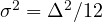 (lesson on quantisation).
The Gaussian distribution

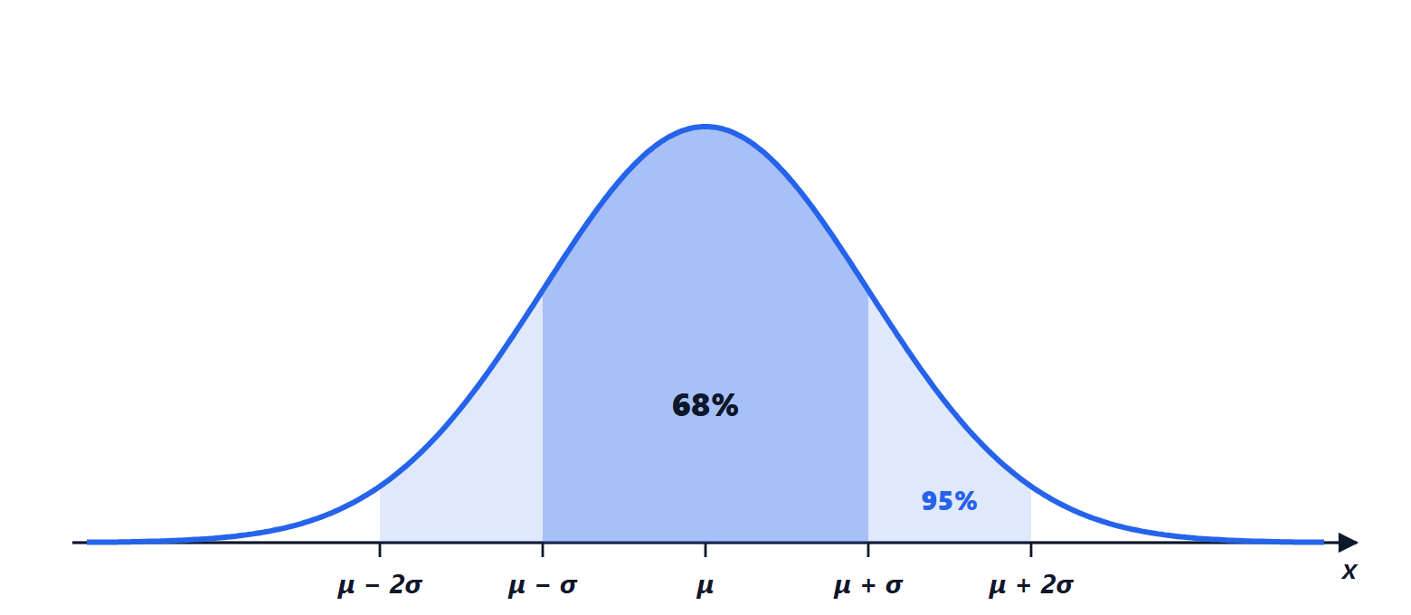
It is determined by mean and variance. Within  of the mean fall 68.3% of the values, within
 95.4%, within
 99.7%. Tails are computed with the function
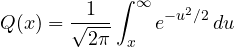
the probability that a standard Gaussian exceeds  : it will be needed for the error probability of transmission systems.
Several variables together
For two variables the joint density  is used. They are independent if
 . The covariance
 measures how much they vary together, and the correlation coefficient
 , between −1 and 1, is its normalised version. Independent implies uncorrelated (
 ); the converse does not hold in general, but it does for jointly Gaussian variables.
Sum of independent variables. If  with and
 independent:
- the means add, always;
- the variances add:
 , because the cross term
 is zero;
- the density of
 is the convolution of the two densities.
The second property is why the powers of independent noises add, while RMS values combine “in quadrature”: two noises of 3 µV and 4 µV give 5 µV.
The central limit theorem
Theorem (statement). The sum of many independent random variables, with finite variances and none dominating the others, has a distribution that tends to the Gaussian, whatever the distribution of the individual variables.
You can see it already by adding a few uniform variables: the convolution of two rectangles is a triangle, of three a bell curve made of parabolas, and after about ten the difference from the Gaussian is tiny. This is why the Gaussian is everywhere in engineering: thermal noise is the sum of the contributions of billions of electrons, measurement errors are the sum of many small causes. So the standard model of noise in communication systems is Gaussian noise, which we study in the next lesson as a random process.




