Discrete-time systems and FIR and IIR digital filters
The convolution sum, difference equations, transfer function and frequency response, poles and zeros, the moving average, the first-order recursive filter and stability with proof.
Once sampled and quantised, a signal is a sequence of numbers  , and the systems that process it are programs: a microcontroller filtering a sensor reading, an audio processor equalising music, a modem demodulating. In this lesson we see how discrete-time systems are described, their frequency response and the two big families of digital filters, FIR and IIR.
Linear discrete-time systems
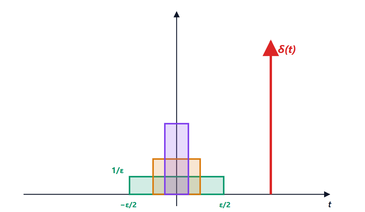
The definitions are those of continuous time with sums instead of integrals. The impulse is  , equal to 1 for
 and 0 elsewhere; the impulse response
 fully describes an LTI system, and the output is the convolution sum
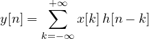
The proof is identical to the continuous-time one:  , then linearity and time invariance. The system is stable if and only if
 .
Difference equations
In practice a digital filter is described by a difference equation: the current output is a combination of the current and past inputs and, possibly, past outputs:

It is literally the program: at each new sample a few multiplications and additions are done. With the Z transform (Mathematical Methods lesson), where a one-sample delay corresponds to multiplying by  , we get the transfer function

The roots of the numerator are the zeros, those of the denominator the poles.
Frequency response
A sampled sinusoid  , with
 the normalised angular frequency, is an eigensignal: the output is
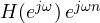 . The frequency response is therefore
 evaluated on the unit circle,
 . Two differences from continuous time:
- it is periodic with period
 : angular frequencies differing by give the same samples (aliasing seen from the other side);
- it is enough to study it for
 , that is from 0 to
 .
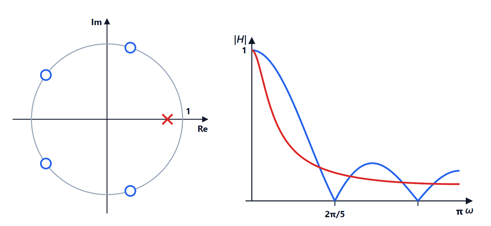
Geometric reading.  is small when the point
 is close to a zero, large when it is close to a pole. From the pole-zero plot one can “see” the filter’s behaviour.
FIR filters
A finite impulse response (FIR) filter uses only the inputs:  , and the impulse response is the sequence of coefficients.
Example: the moving average.  . Summing the geometric series,
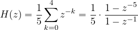
The zeros are the fifth roots of unity except  :
 ,
 . The response vanishes at
 , that is at
 , and at its multiples: it is a simple low-pass that completely removes a disturbance of known frequency. With
 Hz, five samples cover one period of the 50 Hz mains, which disappears from the measurement.
Advantages: they are always stable (they have no poles away from the origin) and, with symmetric coefficients, they have exactly linear phase, that is no phase distortion. Drawback: a steep transition needs many coefficients, even hundreds.
IIR filters
An infinite impulse response (IIR) filter also uses past outputs (it is recursive).
Example: the first-order filter.  , with
 :

One pole at  , unity gain at DC. It is the “exponential moving average” used everywhere to smooth noisy readings, with a single multiplication per sample; with
 the memory is about
 samples. It is the digital equivalent of the RC circuit.
Theorem. A causal LTI system with a rational transfer function is stable if and only if all its poles lie inside the unit circle.
Proof (simple poles). Expanding in partial fractions, the impulse response is a combination of terms  (plus possibly a finite number of impulses). The series
 converges if and only if
 , so
 is finite if and only if all poles have magnitude less than 1. ∎
Advantages: steep transitions with few coefficients; they are designed starting from the classic analogue filters (Butterworth, Chebyshev) with the bilinear transform. Drawbacks: nonlinear phase, and the risk of instability if the coefficients, rounded in finite-precision arithmetic, move a pole outside the circle.
In practice
A digital filter is a loop of a few lines of code:
/* first-order filter with a = 0.8 */
float y = 0.0f;
float filter(float x) {
    y = 0.8f * y + 0.2f * x;
    return y;
}
Digital signal processors (DSPs) have dedicated instructions that perform a multiply and an add in a single cycle, and modern microcontrollers have simplified versions of them. The big advantage over analogue filters is repeatability: no component tolerances, no drift with temperature, and the filter is changed by updating the program.