The DTFT, frequency response and group delay
The discrete-time Fourier transform and its periodicity, exponentials as eigenfunctions with proof, the moving-average response proved, linear phase and group delay, computation with the FFT.
Digital signal processing treats signals as sequences of numbers and transforms them with algorithms: filters, spectral analysis, sample-rate changes. The basis of everything is the frequency-domain description of discrete-time signals and systems. In this lesson we look at the discrete-time Fourier transform (DTFT), the proof that complex exponentials are eigenfunctions of linear systems, the frequency response of the moving average with its proof, and group delay with linear phase. Sampling, convolution and basic FIR and IIR filters are in the Signal Theory lessons; the z-transform and the DFT have lessons of their own.
The discrete-time Fourier transform
For a sequence  , the DTFT is

The variable  is the normalised angular frequency, in radians per sample: a signal sampled at
 with frequency
 has
 . The DTFT is periodic with period
 , because
 for every integer
 : all the information lies in
 , and
 corresponds to half the sampling frequency. It is the z-transform evaluated on the unit circle,
 .
The properties are those of the continuous Fourier transform: convolution becomes product, a delay of  samples multiplies by
 , and Parseval’s theorem holds,
 .
The frequency response
Theorem. If a linear time-invariant system with impulse response  receives the input
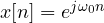 , the output is

Proof. By the convolution sum

∎
A complex exponential goes through the system remaining itself, multiplied by a complex number: it is an eigenfunction. The magnitude  says how much each frequency is amplified, the phase
 how much it is shifted. For a real sinusoid, the sum of two conjugate exponentials, the output is the same sinusoid with amplitude multiplied by
 and phase shifted by
 .
The moving average
The simplest filter averages the last  samples:
 .
Theorem. The frequency response of the moving average is

Proof. It is a geometric series with ratio  :

Factor  out of the numerator and
 out of the denominator:
 , and likewise the denominator. The ratio of the exponentials gives
 and the ratio of the sines the rest. ∎
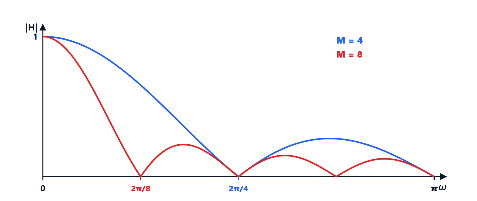
The gain is 1 at DC and vanishes for  : the moving average exactly cancels sinusoids that complete an integer number of periods in samples. It is the same principle as mains rejection in integrating voltmeters (Electrical Measurements lesson on the digital voltmeter). As a low-pass filter, though, it is modest: the side lobes are high, the first around 22 % (−13 dB).
Linear phase and group delay
The phase of the moving average is  , a straight line: all frequencies are delayed by the same number of samples,
 . In general the group delay is defined as
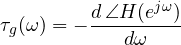
which measures the delay of the envelope of a narrowband signal around . If the phase is linear,  is constant and the waveform passes without phase distortion, only delayed (Signal Theory lesson on distortionless transmission). It is a valuable property for audio, images and digital communications, where phase distortion deforms pulses and creates intersymbol interference. In the next lesson we will see that FIR filters with symmetric coefficients always have linear phase, while IIR filters in general do not.
A note on computation
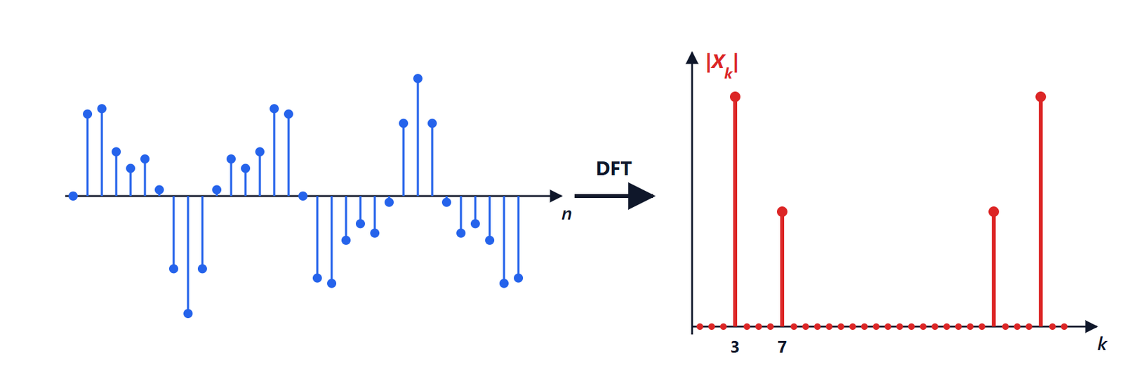
The DTFT is a continuous function of and cannot be computed as such. Samples of it are computed with the DFT, which for an  -point sequence gives
 at the frequencies
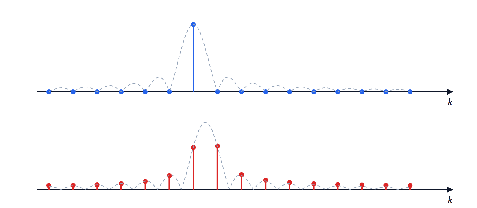
 , and it is computed quickly with the FFT (lesson on the DFT and FFT). To plot a frequency response it is therefore enough to compute the FFT of the impulse response, padded with zeros to get denser points.