FIR filter design with the window method
Impulse response of the ideal low-pass filter with proof, the Gibbs phenomenon, Hann, Hamming and Blackman windows, the Kaiser window with its design formulas, linear phase proved.
The most direct way to design an FIR filter is to start from the ideal filter, compute its impulse response and shorten it. This is the window method: simple, robust and still widely used. In this lesson we derive the impulse response of the ideal low-pass filter, see why truncation creates Gibbs oscillations, compare the classic windows and the Kaiser window with its design formulas, and prove that an FIR filter with symmetric coefficients has linear phase.
The ideal low-pass filter
The ideal low-pass filter has gain 1 for  and 0 elsewhere, in the period
 .
Theorem. Its impulse response is

Proof. With the inverse DTFT formula:

and for  the integral is simply
 . ∎
This response is infinite in both directions and non-causal: no real filter can implement it. So only  central samples are kept and everything is delayed by
 , making the filter causal:
 , where
 is the window, zero outside
 .
The Gibbs phenomenon
Multiplying by the window in time means convolving the ideal response with the window’s transform in frequency. For the rectangular window this transform is the kernel of the previous lesson, with a main lobe  wide and high side lobes. The convolution has two effects:
- a transition band roughly as wide as the main lobe, which narrows as
 increases;
- ripples in the passband and stopband, due to the side lobes. The highest is about 9 % of the jump, and it does not decrease as grows: the ripples become denser but not smaller. This is the Gibbs phenomenon, the same as for truncated Fourier series.
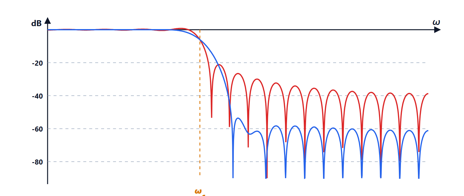
For a filter with the rectangular window the maximum stopband attenuation therefore stays around 21 dB, whatever the length: too little for almost every application.
Windows
The solution is to use windows that taper smoothly to zero at the edges: the side lobes of their transform are much lower, at the price of a wider main lobe, i.e. a slower transition for the same .
| Window | Main lobe width | Highest side lobe | Filter attenuation |
|---|---|---|---|
| rectangular | | −13 dB | 21 dB |
| Hann |  | −31 dB | 44 dB |
| Hamming | | −41 dB | 53 dB |
| Blackman |  | −57 dB | 74 dB |
The Hamming window, for example, is  .
The Kaiser window
Fixed windows force a choice from a table. The Kaiser window has a parameter  that continuously adjusts the trade-off between main-lobe width and side-lobe height, and empirical design formulas. Given the required attenuation
 in decibels (with
 the tolerance, the same in passband and stopband) and the transition width
 :

Example. Passband up to  , stopband from
 with 50 dB. Then
 and
 taps. With the Hamming window, which guarantees the 50 dB, one would need
 , i.e. about 67 taps: the Kaiser window saves a quarter. The cutoff is placed in the middle of the transition,
 .
Linear phase
Theorem. If the coefficients of a length- FIR filter are symmetric,  , then

with  real: the phase is linear and the group delay is
 samples.
Proof. Let  be the centre. Factor out
 :
 . In the sum, the terms
 and
 have the same coefficient and opposite exponents,
 , so together they give
 , which is real. If is odd the central term
 remains, also real. So the sum is a real number . ∎
can change sign, and then the phase jumps by  : it is still piecewise linear, and the group delay is constant. A filter designed with windows is symmetric by construction (the centred ideal response and the windows are even), so it always has linear phase. This is the main advantage of FIR filters over IIR ones, together with guaranteed stability: an FIR filter has no poles away from the origin.