Multirate processing: decimation, interpolation and polyphase filters
Spectrum of the downsampled signal with proof, the decimator, upsampling and images, rational rate conversion, the noble identity proved, the polyphase structure, sigma-delta converters and software radio.
Many systems work with different sampling rates at different points: an oversampled converter produces millions of samples per second that must be reduced, audio goes from 44.1 to 48 kHz, a digital radio extracts a narrow channel from a wide band. Multirate processing changes the sampling rate numerically. In this lesson we prove what happens to the spectrum when downsampling and upsampling, look at the filters needed, rational rate conversion, and the polyphase structure with the noble identities that make it all efficient.
Downsampling
Downsampling by an integer factor  means keeping one sample every :
 .
Theorem. The spectrum of the downsampled signal is
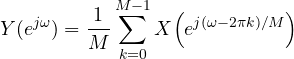
Proof. Introduce the intermediate signal  , where
 is 1 when
 is a multiple of and 0 otherwise. This comb can be written as an average of exponentials,
 (the sum is if is a multiple of and 0 otherwise, by the geometric series). Multiplying by
 shifts the spectrum by
 , so
 . Finally
 only removes zeros, and its transform is
 . Substituting gives the formula. ∎
The spectrum is stretched times and shifted copies are added. If the original signal had components above  , the copies overlap: this is aliasing, and it can no longer be removed.
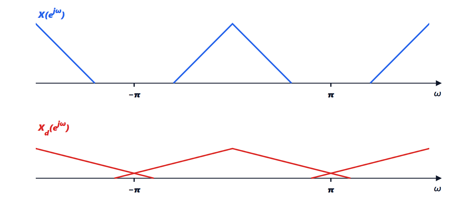
That is why, before downsampling, the signal is filtered with a low-pass filter at : filter plus downsampler together are called a decimator.
Upsampling
Upsampling by a factor  means inserting
 zeros between samples:
 if is a multiple of , 0 otherwise. The spectrum is
 , because only the terms
 remain in the transform sum, with
 . The spectrum is compressed times, and copies appear in the interval
 : the images. A low-pass filter at
 with gain removes them and fills the zeros with interpolated values: this is the interpolator.
Rational rate conversion
To multiply the sampling rate by  , upsample by , filter with a single low-pass filter with cutoff
 , which removes the images and prevents aliasing at the same time, and downsample by . Converting from CD audio (44.1 kHz) to professional audio (48 kHz) has ratio
 : upsampling by 160 followed by downsampling by 147. Done literally it would be an enormous computation, at 7 MHz in the middle; polyphase structures make it practical.
The noble identities and the polyphase structure
The obvious flaw of the decimator is that the filter works at the high rate and then  samples out of are thrown away: most multiplications are wasted.
Theorem (noble identity). Filtering with  and then downsampling by is equivalent to downsampling by and then filtering with
 .
Proof. has an impulse response that is non-zero only at multiples of :  . The filter output at instant
 is
 , which is exactly the convolution of
 with the downsampled signal
 . ∎
Every FIR filter  can be split into polyphase components, collecting the coefficients with index
 :
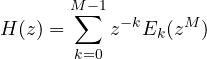
Applying the noble identity to each branch, the downsampling moves before the filters  , which work at the low rate. The number of multiplications per output sample is still that of the filter, but the number per unit time drops by a factor . The same holds, dually, for the interpolator. For the 160/147 conversion only the output samples that are needed are computed, each time using the right subset of coefficients.
Applications
- Oversampled converters. A sigma-delta converter samples at many megahertz with few bits and pushes the quantisation noise to high frequencies; a digital decimator filters it out and reduces the rate, gaining bits (Applied Electronics lesson on converters). The first stages often use CIC filters, cascades of integrators and differentiators that need no multiplications.
- Software-defined radio. A wide band is sampled, the desired channel is brought to baseband with a numerical oscillator and decimated down to the channel width.
- Filter banks. A signal is split into sub-bands, each downsampled and coded with the appropriate number of bits: this is the basis of audio compression (MP3, AAC) and of the polyphase banks of OFDM.