The real op-amp: finite gain, gain-bandwidth product, slew rate and offset
Effect of finite gain, dominant pole and gain-bandwidth product with proof, slew rate and full-power bandwidth, offset, bias currents, CMRR and rail-to-rail.
The ideal op-amp is an excellent model, but real components have finite gain, limited bandwidth, a maximum rate of change of the output and small DC errors. Choosing the right op-amp for an application means knowing which of these limits matters. In this lesson we cover the effect of finite gain, the gain-bandwidth product, slew rate and offset errors, with the numbers found on datasheets.
Finite gain
With finite gain  and a fraction
 of the output fed back to the input, the gain of the non-inverting amplifier is

(we derive it in the lesson on feedback). For  the ideal value
 is recovered. The product
 , the loop gain, measures how close we are to the ideal: the relative error is about
 .
Example.  , desired gain 10 (
 ):
 , an error of 0.01%, far less than the resistor tolerance.
The gain-bandwidth product
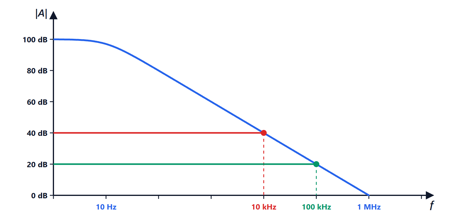
The gain is very high only at very low frequencies. Almost all op-amps are internally compensated: they have a dominant pole at a few hertz, after which the gain falls by 20 dB per decade:
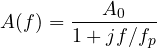
For  ,
 : the product of gain and frequency is constant. It is the gain-bandwidth product (GBW), the frequency at which the open-loop gain equals 1.
Theorem. An amplifier with ideal gain  built with an op-amp of gain-bandwidth product GBW has bandwidth
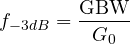
Proof. Substituting  (valid above
 ) into
 :

a first-order system with gain  and cut-off frequency
 . ∎
Example. With GBW = 1 MHz, an amplifier with gain 10 reaches 100 kHz, with gain 100 only 10 kHz. If gain 100 and 100 kHz bandwidth are needed, either a 10 MHz op-amp is chosen or two gain-of-10 stages are cascaded.
Slew rate
The output cannot change faster than a maximum value, the slew rate  (in V/µs), set by the current with which the internal stages charge the compensation capacitance. A sinusoid
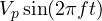 has a maximum slope of
 , so it passes undistorted only if

Example. A cheap op-amp with  V/µs, with a 10 V peak output, already distorts above
 kHz, even though its GBW would allow much more. Large-signal audio needs a few V/µs; video signals hundreds.
DC errors
- Offset voltage
 : even with both inputs at the same voltage the output is not zero, as if a small source were in series with the input (from microvolts to a few millivolts). It is amplified by the gain : 2 mV of offset with a gain of 100 gives 200 mV at the output.
- Bias currents
 : the inputs draw a small current (nanoamperes for bipolar op-amps, picoamperes for MOSFET or JFET ones), which flowing through the resistors produces further error voltages. It is partly compensated by placing on the non-inverting input a resistor equal to the parallel combination of those on the inverting input.
- Drift with temperature, in µV/°C: often more important than the offset itself, which can be trimmed.
For precision measurements on small signals there are chopper or zero-drift op-amps, which continuously correct their own offset down to a few microvolts.
Other parameters
| Parameter | Meaning | Typical values |
|---|---|---|
| CMRR | how much a voltage common to both inputs is rejected | 80-120 dB |
| PSRR | how much supply variations reach the output | 80-110 dB |
| noise | input-referred noise voltage | 1-50 nV/√Hz |
| output swing | how close the output gets to the supplies | from 1-2 V to a few mV (rail-to-rail) |
| output current | maximum current that can be delivered | 10-50 mA |
Rail-to-rail op-amps get within a few millivolts of the supplies, essential with the low supplies (3.3 V or less) of modern circuits. There is no single best op-amp: fast ones often have more offset and draw more current, precise ones are slow. The choice always starts from the parameter that limits the application.