The ideal op-amp: inverting, non-inverting and adder
The ideal op-amp and the virtual short, inverting and non-inverting amplifiers with proof, follower, adder, difference amplifier and a design example.
The operational amplifier is the most widely used analogue component: a differential amplifier with enormous gain that, on its own, is almost unusable, but with two feedback resistors becomes a precise amplifier, an adder, a filter, an integrator. Its behaviour is computed with two very simple rules. In this lesson we derive them and apply them to the fundamental configurations.
The ideal op-amp
An op-amp has two inputs, inverting (−) and non-inverting (+), and one output:

The ideal op-amp has infinite gain  , infinite input impedance (it draws no current from its inputs), zero output impedance and infinite bandwidth. Real ones come close: between
 and
 , input currents of nanoamperes or picoamperes.
The virtual short
The two rules. If the op-amp is connected with negative feedback (part of the output returns to the inverting input) and is not saturated:
- the input currents are zero;
 : there is a virtual short between the two inputs.
Why. The first is the definition of infinite input impedance. For the second: the output is finite (limited by the supply), so  tends to zero as
 . Negative feedback is what sets the output at exactly the value that makes the difference zero: if
 exceeds
 , the output falls and brings back down. Without negative feedback the rule does not hold: the output goes to one of its two extremes (comparator operation).
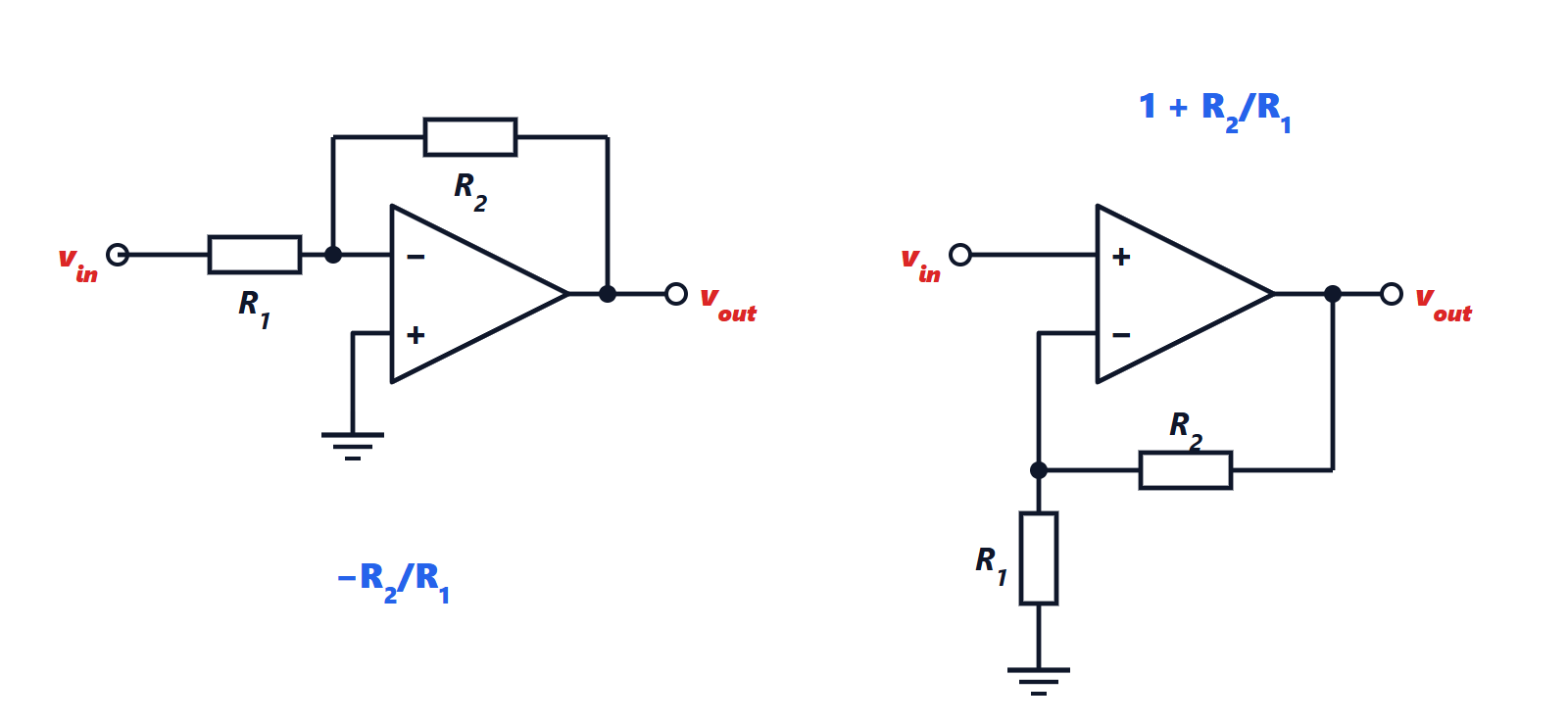
The inverting amplifier
Theorem. 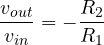 , and the input impedance is
 .
Proof. The non-inverting input is grounded, so by the virtual short  (a virtual ground). The current in is
 ; since it cannot enter the op-amp, it all flows on through
 :
 . The gain follows. The input source sees towards a point at zero potential, so the input impedance is . ∎
The gain depends only on the ratio of two resistors, not on the op-amp: with 1% resistors the gain is accurate to 1 to 2%, whatever the value of and its drift with temperature.
The non-inverting amplifier
Theorem. 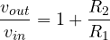 , with (ideally) infinite input impedance.
Proof. By the virtual short  . The inverting input is connected to the output through the – divider:
 . Equating gives the gain. The signal goes straight into the input, which draws no current. ∎
The voltage follower. With  (output connected directly to the inverting input) and no , the gain is 1. It looks useless, but it is invaluable: it copies the voltage of a source that cannot supply current (a sensor, a high-impedance divider) onto any load. It is a buffer.
Adder and difference amplifier
Inverting adder. Several inputs, each with its own resistor  , into the same virtual-ground node: the currents add up in
 , and

With equal resistors it is a sum, with different weights a weighted sum: the principle of audio mixers and digital-to-analogue converters.
Difference amplifier. With four resistors ( and on the inverting input as in the inverting amplifier, and an – divider on the non-inverting input), by superposition
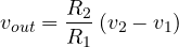
It amplifies the difference between two voltages and ignores what they have in common. It is the basis of bridge-sensor measurements and of instrumentation amplifiers, which we will see in the lesson on linear circuits.
Example. A sensor produces 0 to 100 mV and the analogue-to-digital converter accepts 0 to 3.3 V. A gain of 33 is needed: a non-inverting amplifier with  kΩ and
 kΩ, or, with standard values,
 kΩ (gain 34, full scale at 3.4 V, slightly beyond: one picks 31.6 kΩ from the 1% series).
The limits
The two rules are excellent approximations as long as the required gain is much smaller than at the operating frequency, the output stays within the supplies and the current drawn from the output is within the component’s limits. The next lesson says what happens when these conditions fail.