Fluids in plants: Bernoulli, pressure losses and pumps
Stevin's law with proof, conservation of mass, Bernoulli's equation from the energy balance, the Venturi tube, the Darcy-Weisbach formula with an example, choosing the pump.
Thermal plants move fluids: water in heating and cooling circuits, air in ventilation ducts, liquid coolants in servers. Sizing pipes, pumps and fans requires a few principles: fluid statics, conservation of mass, Bernoulli’s equation and pressure losses. In this lesson we derive them, linking them to the energy balance of the first lesson.
Fluid statics
In a fluid at rest pressure grows with depth (Stevin’s law):

Proof. Consider a small vertical column of fluid of cross-section  and height
 . It is in equilibrium: the pressure force below must support the one above plus the weight,
 , that is
 . With constant
 , integrate. ∎
Example. Ten metres of water produce  kPa, almost one atmosphere: that is why the heating system of a ten-storey building runs at a few bar at the bottom.
Conservation of mass
For a liquid in a duct, in steady state, the volume flow rate is the same at every section:  . Where the duct narrows the fluid speeds up, where it widens it slows down.
Bernoulli’s equation
Theorem. Along a duct, for an ideal liquid (incompressible, frictionless, with no heat or work exchange), in steady state:

Proof. Apply the open-system energy balance (first lesson) between two sections, with  and
 :
 . For an incompressible liquid
 , and without friction or heat the internal energy does not change:
 . Substituting and multiplying by gives the statement. ∎
The three terms are static pressure, dynamic pressure and potential energy per unit volume. Divided by  they become heads (in metres of fluid column), a very common way of expressing them in plants.
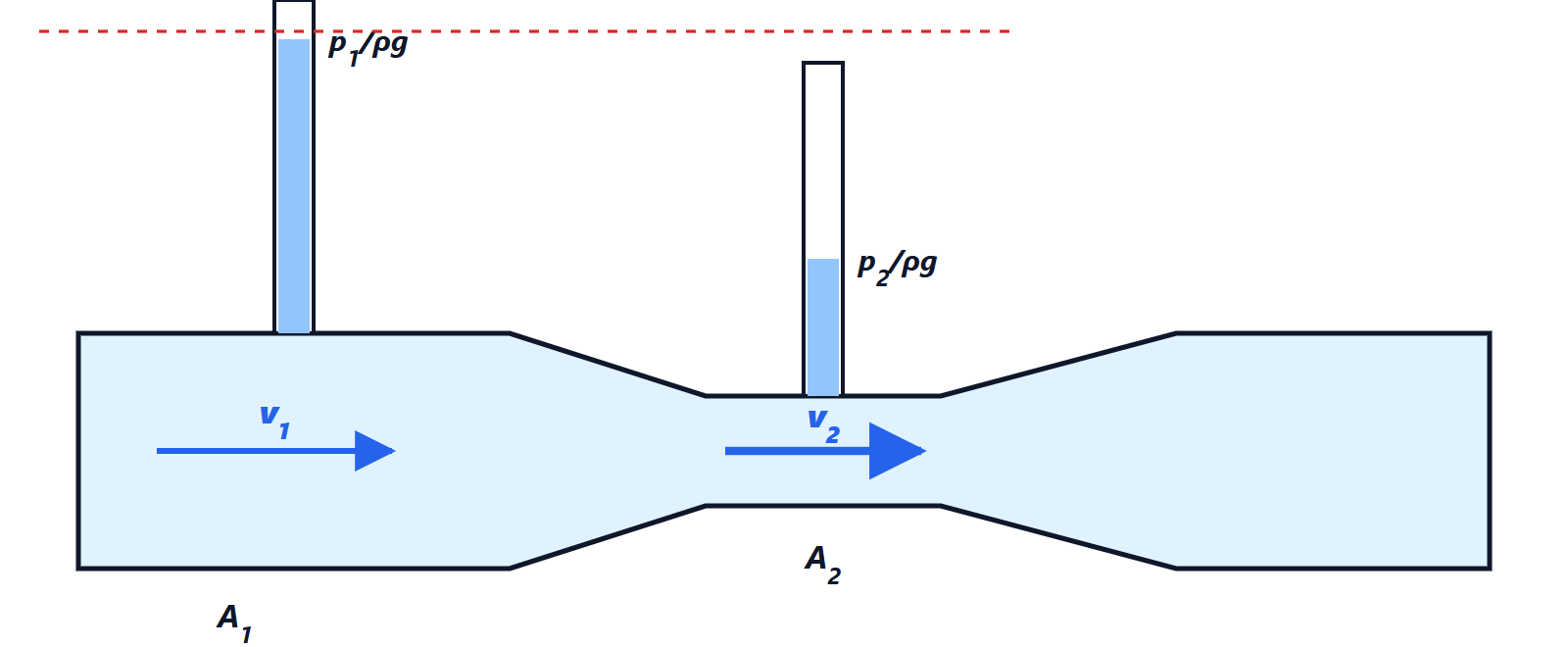
The Venturi tube. In the throat the velocity increases and therefore, by Bernoulli, the pressure decreases. Measuring the pressure difference between the two sections gives the velocity, and hence the flow rate: 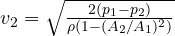 . It is one of the most widely used flow meters; the same principle explains the Pitot tube that measures aircraft speed and how old carburettors worked.
Pressure losses
In real fluids friction with the walls and turbulence dissipate energy, and the Bernoulli sum decreases along the path. The loss in a straight pipe is given by the Darcy-Weisbach formula:
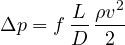
where  is the friction factor. It depends on the Reynolds number
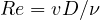 :
- laminar flow (
 ):
 , the fluid flows in orderly layers;
- turbulent flow (
 ): also depends on the pipe roughness, is read from the Moody chart, and is typically between 0.015 and 0.04.
Bends, valves and fittings add minor losses,  , with tabulated coefficients
 .
Example. Water at 2 m/s in a 5 cm diameter pipe, 100 m long. With  m²/s,
 : turbulent flow,
 . The loss is
 kPa, about 8 m of water column. The flow rate is
 litres per second, and the hydraulic power the pump must supply to make up the loss is
 W (more in electrical terms, divided by the pump efficiency).
Choosing the pump
The pressure lost grows with the square of the velocity, hence of the flow rate: the system has a parabolic characteristic curve. The pump has its own curve, with pressure falling as flow increases. The operating point is the intersection of the two, exactly like the load line and a transistor’s characteristic in the lesson on amplifiers. Doubling the pipe diameter, for the same flow, cuts the velocity fourfold and the loss by about 32 times: that is why large plants favour big pipes and small pumps, which use less energy over the whole life of the plant.