Spectral analysis: leakage, windows, periodogram and Welch's method
DFT of a finite block and spectral leakage proved, resolution, dynamic range and scalloping loss, zero padding with proof, the periodogram, Welch's method and variance reduction, the spectrogram.
Computing the spectrum of a measured signal looks easy: take a block of samples and compute the FFT. But the result depends on how the block was cut, and on a noisy signal it is surprisingly unreliable. In this lesson we look at spectral leakage with its proof, resolution and scalloping loss, why zero padding does not increase resolution, the periodogram and Welch’s method with the proof of the variance reduction, and the spectrogram.
The DFT of a finite block
When  samples are analysed the signal is observed through a rectangular window, and the DFT gives samples of the DTFT of the windowed signal, at the frequencies
 (the bins). With sampling frequency
 the bins are
 apart: with 1 kHz and 1000 samples, 1 Hz.
Theorem. For 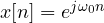 ,
 , the DFT is

If  coincides with a bin,
 , the DFT is in bin
 and zero in all the others; otherwise it is non-zero in every bin.
Proof. It is the same geometric series as the moving average (lesson on the DTFT), with ratio  . If , for
 one has
 , a multiple of
 : the sine in the numerator is zero while the one in the denominator is not. For
 all the terms equal 1. If falls between two bins,
 is never a multiple of and no term vanishes. ∎
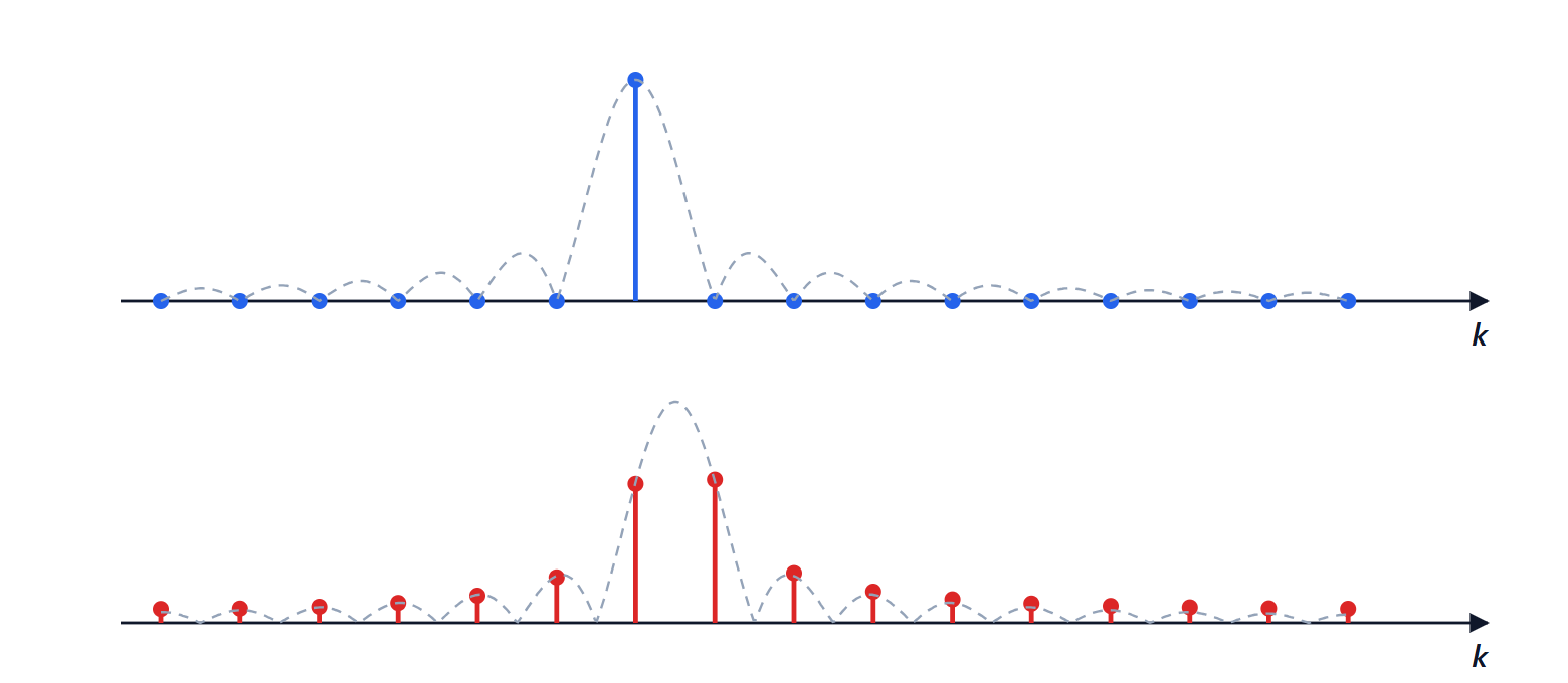
This is spectral leakage: a pure sinusoid appears as a peak surrounded by a “skirt” spreading over the whole spectrum, falling off slowly (the side lobes of the rectangular window, the first at −13 dB). The physical reason is that the DFT treats the block as one period of a periodic signal: if the number of periods is not an integer, there is a jump at the junction, and a jump has a wide spectrum.
Resolution, dynamic range and scalloping loss
The consequences are managed with the windows of the FIR lesson, applied this time to the signal:
- resolution: two sinusoids can be told apart if they are farther apart than the main-lobe width, about
 for the rectangular window and
 for Hann and Hamming. Resolving close frequencies requires long blocks;
- dynamic range: a weak sinusoid near a strong one stays hidden in the latter’s side lobes. Windows with low side lobes (Hann, Blackman, Kaiser) make it possible to see components 60-100 dB below;
- scalloping loss: if the frequency falls halfway between two bins, the measured peak is lower. With the rectangular window the value is
 , i.e. −3.9 dB. Flat-top windows reduce it below 0.01 dB and are used to measure amplitudes accurately.
Zero padding does not increase resolution
Extending the block with zeros before the FFT (zero padding) produces a denser, smoother plot, but it does not separate two close sinusoids.
Theorem. The  -point DFT (
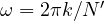
 ) of the zero-padded block gives samples of the same DTFT as the original block, at the frequencies
 .
Proof.  , because the added samples are zero; and this is the DTFT of the original block evaluated at
 . ∎
The sampled function is always the same, with the same main lobe: zero padding interpolates, useful to read the position of a peak better, but the information is that of the measured samples.
The periodogram and Welch’s method
For a random signal, such as noise, what matters is the power spectral density (Signal Theory lesson on random processes). The immediate estimate is the periodogram  . It has a serious flaw: its standard deviation in each bin is of the order of the value itself, and it does not decrease as the block gets longer. More samples give more bins, but each one stays just as noisy: the estimated spectrum of white noise looks like dense grass instead of a flat line.
Welch’s method divides the signal into  segments (often overlapping by 50 %), applies a window to each, computes its periodogram and averages.
Theorem. If the periodograms are independent and have the same variance  , their average has variance
 .
Proof. It is the same result as the mean of  readings (Electrical Measurements lesson on uncertainty):
 . ∎
The price is resolution: each segment is times shorter. It is the fundamental trade-off of spectral analysis: resolution versus variance, for a given signal duration. Digital spectrum analysers do exactly this, averaging many FFTs.
The spectrogram
For signals that change over time, such as speech or music, the DFT is computed on successive windows and the results are placed side by side: this is the spectrogram (short-time Fourier transform, STFT). A long window gives good frequency resolution but blurs fast events; a short one the opposite. The product of the two resolutions cannot go below a limit, as in the uncertainty principle:  is at least of the order of 1. Wavelet transforms choose long windows for low frequencies and short ones for high frequencies, adapting to many natural signals.