Finite differences for partial differential equations: heat, stability and CFL
Derivatives as differences, the explicit scheme for the heat equation, the stability condition, Crank-Nicolson, Lax-Richtmyer, the Courant condition and FDTD.
The partial differential equations of the Mathematical Methods lesson can be solved by hand only on simple domains. For a heat sink of realistic shape, for the field in a semiconductor device, for a signal travelling on a line with discontinuities, numerical methods are needed. The most direct is the finite difference method: space and time are replaced by a grid of points and derivatives by difference quotients. In this lesson we apply it to the heat equation and look at consistency, stability and convergence, and at the Courant condition for waves.
Derivatives as differences
From Taylor’s expansion, with step  :

The second, centred, is more accurate for the same step, because the errors of the two sides cancel. For the second derivative, adding the expansions at  and
 :

with error  . These formulas are enough to discretise almost every equation in physics.
The heat equation: the explicit scheme
 on
 . Introduce the grid
 ,
 , and write
 for the approximation of
 . Using a forward difference in time and a centred one in space:

that is, with  ,

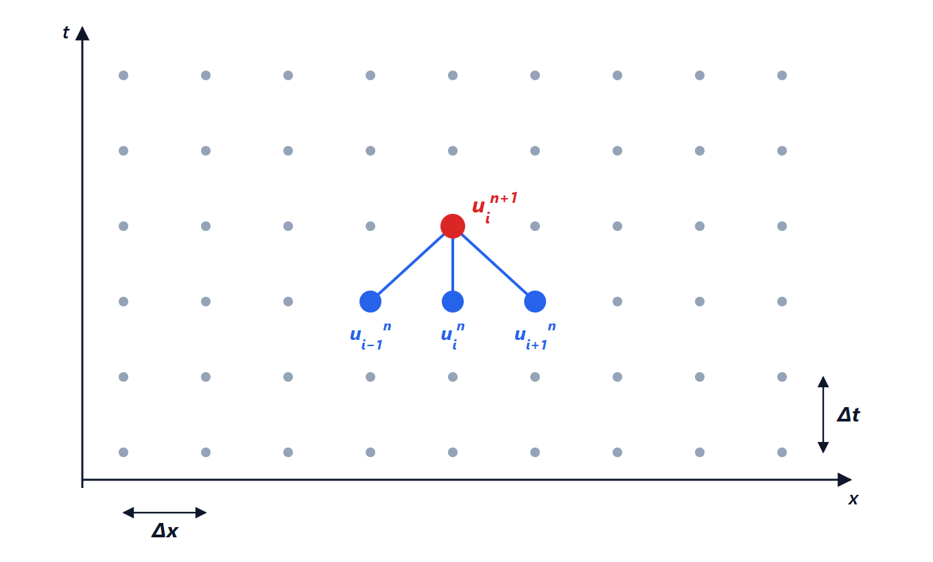
 (red) is computed from the three neighbouring values at the previous step (blue): the “stencil” of the explicit scheme.
Each new value is computed from its three neighbours at the previous step: start from the initial condition and advance row by row, applying the boundary conditions at the ends. It can be programmed in a few lines, even in a spreadsheet.
Stability: 
The scheme is stable only if
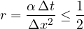
Why. With  the new value is a weighted average of the three neighbours with positive weights,
 : it cannot exceed the largest of the old values, so errors do not grow (discrete maximum principle). With
 the central weight becomes negative, and a small point-to-point oscillation is amplified at every step: after a few dozen steps the solution blows up into a meaningless zigzag.
The practical consequence is heavy: halving for more detail means dividing  by four, and the total work grows eightfold. As with stiff differential equations, the answer is implicit schemes: the Crank-Nicolson scheme, which averages the old and new steps, is stable for any and has error
 . At each step it needs to solve a tridiagonal linear system, which is cheap.
Consistency, stability, convergence
- A scheme is consistent if, as the steps tend to zero, the discrete equation tends to the true one (the truncation error goes to zero).
- It is stable if errors, from rounding or from the data, do not grow without bound over the steps.
- It is convergent if the numerical solution tends to the true one as the steps tend to zero.
The Lax-Richtmyer equivalence theorem states that for well-posed linear problems a consistent method is convergent if and only if it is stable. It is the central result of the whole theory, and it is the one referred to in the introduction to finite difference methods linked to this subject.
The wave equation and the Courant condition
For  , with centred differences in time and space, the explicit scheme is stable if and only if
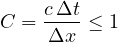
the Courant-Friedrichs-Lewy (CFL) condition. Its meaning is physical: in one step the wave travels  , and the scheme uses only points a distance away. If the wave travels further than one grid point per step, the scheme cannot “see” where the information is coming from and the solution becomes unstable. The numerical domain of dependence must contain the physical one.
It is the condition that governs FDTD (finite-difference time-domain) electromagnetic simulators, used to design antennas, waveguides and high-speed printed circuit boards: with 1 mm cells and the speed of light, the time step must stay below about 2 picoseconds in three dimensions.
Two dimensions and beyond
For Laplace’s equation on a plate, the difference formula in both directions gives

each value is the average of its four neighbours, the discrete version of the mean value property of harmonic functions. Repeating this averaging over the whole grid until the values stop changing is the Jacobi method of the lesson on linear systems. For complicated geometries, with curved edges, the finite element method is preferred, which splits the domain into triangles or tetrahedra and uses Gaussian quadrature: it is the method of the structural, thermal and electromagnetic simulation programs used in industry.