Linear systems on a computer: LU, pivoting, Cholesky and iterative methods
LU factorisation and its cost, partial pivoting with an example, Cholesky, sparse matrices, Jacobi and Gauss-Seidel methods, spectral radius and the residual.
In Geometry and Algebra linear systems were solved with Gaussian elimination on 3×3 matrices. In real problems matrices have thousands or millions of rows: simulating an integrated circuit, finite element structural analysis, reconstructing an image in a CT scan. What matters here is the cost of the computation, stability with respect to rounding and the structure of the matrix. We look at direct methods (LU and Cholesky factorisations) and iterative ones (Jacobi and Gauss-Seidel).
LU factorisation
Gaussian elimination, recording the multipliers used, splits the matrix into the product

with  lower triangular (1s on the diagonal and the multipliers below) and
 upper triangular (the echelon form). The system
 becomes two triangular systems, solved by substitution:

The advantage. The factorisation costs about  operations, but the two substitutions only
 . If many systems with the same matrix and different right-hand sides must be solved (as in a simulator where only the sources change at each step), you factorise once. With
 :
 operations for the factorisation,
 for each new right-hand side.
Example.

The multipliers 2 and 4 eliminate the first column, the 3 the second.
Pivoting
If a zero appears on the diagonal during elimination the method stops; if a very small number appears, you divide by it and rounding errors blow up.
Example. With 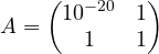 and
 , the true solution is about
 . Without swaps the multiplier is
 , and in double precision the second row becomes
 because
 rounds to
 : you get
 and then
 , completely wrong. Swapping the rows before eliminating gives the correct result.
Partial pivoting chooses at each step, as pivot, the entry of largest magnitude in the column, and swaps rows. The multipliers then have magnitude at most 1 and the method is stable in practice. The factorisation becomes  , with
 a permutation matrix. It is the standard method of every numerical library (LAPACK, NumPy, MATLAB).
Symmetric positive definite matrices: Cholesky
If  is symmetric and positive definite (like structural stiffness matrices, covariance matrices, nodal matrices of resistor-only circuits), then

with lower triangular. The Cholesky factorisation costs half as much as LU ( ), needs no pivoting and is always stable. If the square root of a negative number appears during the calculation, the matrix was not positive definite: it is also the fastest way to check.
Sparse matrices
In applications, large matrices are almost all zeros: in a circuit’s nodal matrix, each row has non-zero entries only for directly connected nodes. A full  matrix would take 8 terabytes in double precision; sparse, with 10 entries per row, 80 megabytes. Sparse direct methods reorder rows and columns to limit fill-in, the zeros that become non-zero during elimination. This is what SPICE and finite element programs do.
Iterative methods
For huge sparse matrices it is often better to start from an estimate  and improve it, without ever factorising.
Jacobi. From equation  solve for
 using the previous iteration’s values for the other unknowns:
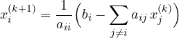
Gauss-Seidel. Like Jacobi, but it uses the values already updated in the same iteration straight away. It usually converges about twice as fast and uses less memory.
Example.  ,
 (solution
 ,
 ). Gauss-Seidel from
 :
 ,
 ; then
 ,
 ; then
 ,
 . Three steps, three correct digits.
When they converge
Writing the iteration as  , the error is multiplied by
 at each step, so the method converges if and only if the spectral radius of (the largest magnitude of its eigenvalues, Geometry and Algebra lesson) is less than 1. A sufficient condition that is easy to check: the matrix is diagonally dominant,
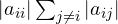 for every row. The nodal matrices of resistive circuits almost always are.
For the largest problems more sophisticated iterative methods are used, such as the conjugate gradient method for symmetric positive definite matrices, which in exact arithmetic reaches the solution in at most  steps and in practice needs far fewer, especially with a good preconditioner.
The residual is not enough
After computing  , the residual
 is easy to compute, but a small residual does not guarantee an accurate solution. The relative error is bounded by
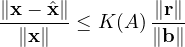
with  the condition number of the lesson on errors. If is large, even a tiny residual can hide a large error.