Numerical integration: trapezoidal, Simpson, Romberg and Gauss
Trapezoidal and Simpson's rules with their errors, a numerical example, Richardson extrapolation, adaptive integration, Gaussian quadrature and sampled signals.
Many integrals have no antiderivative expressible with elementary functions ( ,
 , the perimeter of an ellipse), and often the function is known only at points, like the samples of a signal. Numerical integration (or quadrature) approximates the integral by a weighted sum of the function’s values at a few points. It is how a multimeter computes the RMS value of a voltage, how an electronic meter computes the energy used and how the area under an experimental curve is estimated.
The common idea
Split  into
 intervals of width
 , with nodes
 , approximate
 on each interval with a polynomial and integrate the polynomial exactly.
The trapezoidal rule
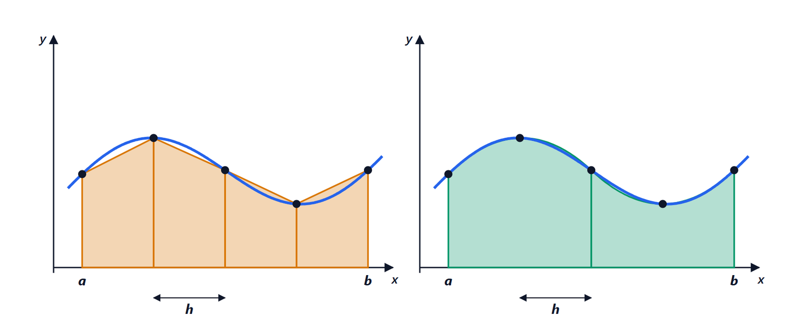
On each interval is replaced by the segment between the two ends, and the area is that of a trapezium. Adding up:

The error is

proportional to  : halving the step cuts the error by four. The rule is exact for first-degree polynomials. The sign of the second derivative tells which side the error is on: for a convex function the trapezia lie above the curve and overestimate the integral.
Simpson’s rule
With even, on each pair of intervals is replaced by the parabola through the three points. Integrating the parabola gives the weights  , and adding up:

The error is
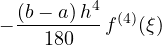
proportional to  : halving the step cuts the error by sixteen. Surprisingly the rule is exact for cubic polynomials too, not just parabolas: the error of the cubic term cancels by symmetry.
Example.  With
 (
 ):
| Method | Value | Error |
|---|---|---|
| trapezoidal | 0.742984 |  |
| Simpson | 0.746855 |  |
With the same five function values, Simpson is more than a hundred times more accurate.
Proof: Simpson from the trapezoidal rule
The trapezoidal error has the form  . Computing with steps
 and
 and combining to remove the term:
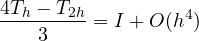
and working it out gives exactly Simpson’s rule. This is Richardson extrapolation: knowing how the error behaves, you can remove it. Repeating the idea gives Romberg’s method, which reaches high accuracy with few values.
Estimating the error without the derivative
The error formulas contain unknown derivatives. In practice the result is compared at two different steps: for the trapezoidal rule,  . Adaptive integration programs do this on each subinterval, and add points only where the function changes quickly: few points where it is flat, many near a peak.
Gaussian quadrature
The trapezoidal and Simpson rules use equally spaced nodes. If the node positions can be chosen too, points can integrate a polynomial of degree  exactly: the Gauss-Legendre formulas. With just two points at
 on
 :

exact for every cubic polynomial, like Simpson but with one point fewer. The nodes are the roots of the Legendre polynomials. These formulas are used in finite element programs, where every function evaluation is expensive.
Integrals of sampled signals
For a signal sampled with period  the nodes are fixed by the converter, and the trapezoidal rule or Simpson is applied to the samples. Example: the RMS value of a voltage,
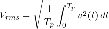
is computed in “true RMS” multimeters by summing the squared samples over a period. For a periodic signal sampled over a whole number of periods, the trapezoidal rule is surprisingly accurate: the error falls faster than any power of , because the end errors cancel. It is the same reason the DFT computes the Fourier coefficients of band-limited signals exactly.
Improper integrals and singularities
On infinite intervals the interval is truncated where the function is negligible, or a change of variable makes it finite. If the function has an integrable singularity, such as  at 0, formulas with nodes at the ends fail (
 is infinite) and convergence is slow: it pays to remove the singularity with a change of variable (here
 ) before integrating.