Interpolation: Lagrange polynomial, Runge's phenomenon, Chebyshev nodes and splines
Existence and uniqueness of the interpolating polynomial, interpolation error, Runge's phenomenon, Chebyshev nodes, linear and cubic splines and their uses.
Often a function is known only at certain points: the values in a table, the measurements of an experiment, the samples of a signal, the characteristic curve of a sensor supplied by the manufacturer. Interpolating means building a simple function that passes exactly through those points, to estimate the values in between. In this lesson we look at the interpolating polynomial, Runge’s phenomenon which shows its limits, Chebyshev nodes and splines.
The interpolating polynomial
Given  points
 with distinct abscissas, there is exactly one polynomial of degree at most
 through all of them.
Proof of uniqueness. If two polynomials  and
 of degree at most pass through the same points, the difference
 has degree at most and vanishes at distinct points. A non-zero polynomial of degree has at most roots, so
 .
The Lagrange form. Build the basis polynomials
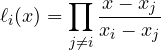
which equal 1 at  and 0 at every other node. Then
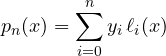
passes through all the points. Example: for  ,
 ,
 one gets
 . The Lagrange form is elegant for proofs; for calculations the Newton form with divided differences is used, which lets you add a point without recomputing everything.
The interpolation error
If  has continuous derivatives, for every
 there is
 in the interval such that

The error depends on two factors: how “smooth” the function is (the high-order derivative) and how the nodes are spread (the product).
Runge’s phenomenon
It seems natural that more points always give a better interpolation. They do not. In 1901 Runge studied the function

perfectly smooth, and interpolated it at equally spaced nodes.
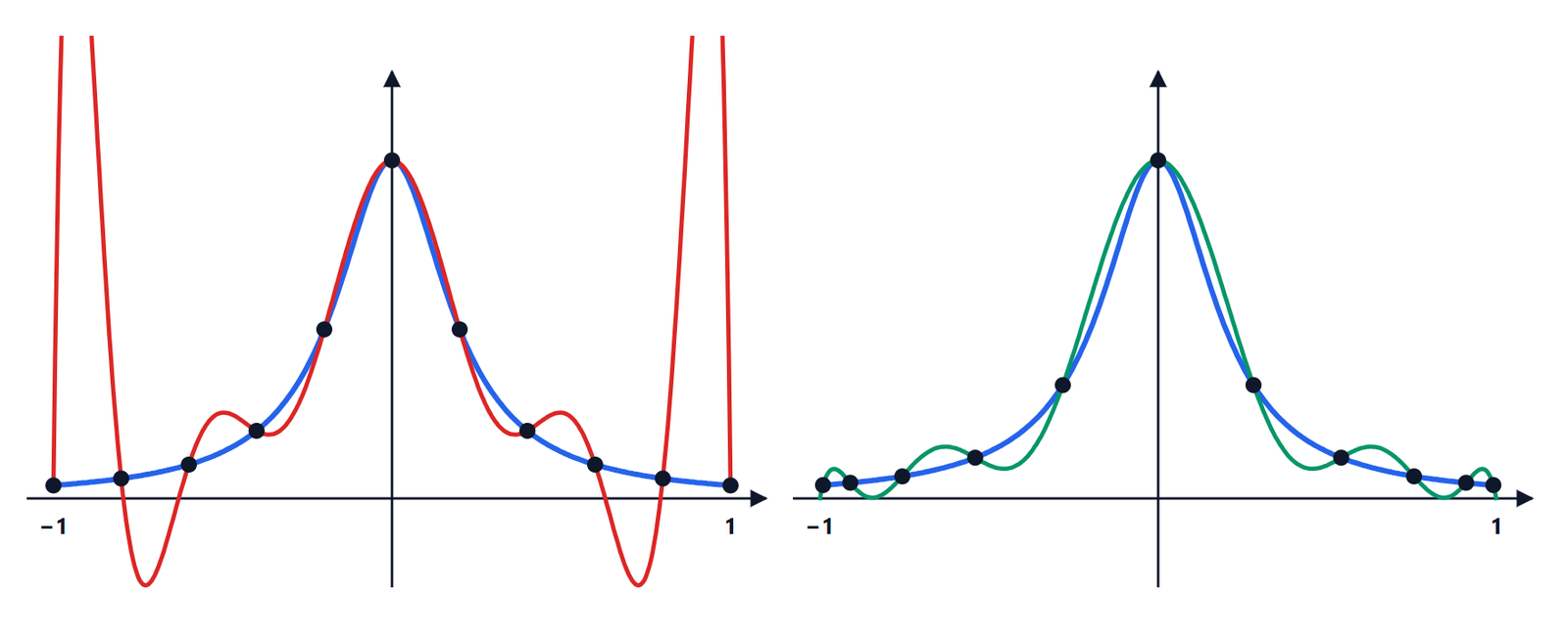
With equally spaced nodes, as the degree rises the error near the ends grows without limit: with 21 nodes the polynomial reaches values above 50, while the function stays between 0 and 1. The cause is the product  , which with equally spaced nodes is much larger near the ends than in the middle. (The deep reason is complex, in the sense of complex numbers: has poles at
 , close to the interval.)
The practical lesson: do not use high-degree polynomials on equally spaced nodes. It is the same reason a degree-10 polynomial fit to experimental data produces curves with absurd wiggles between the points.
Chebyshev nodes
If the nodes can be chosen, it pays to cluster them towards the ends. The Chebyshev nodes on  are

the projections onto the axis of equally spaced points on a semicircle. They make the product  as small as possible (at most
 ), and with them the interpolation of smooth functions always converges. It is the principle numerical libraries use to approximate mathematical functions.
Splines
The most used alternative in practice is to interpolate piecewise: a low-degree polynomial between each pair of nodes, joined smoothly.
- Piecewise linear: the points are joined with segments. Simple and free of oscillations, but with corners. It is what a spreadsheet does with a line chart, and a lookup table in a microcontroller.
- Cubic spline: between two nodes a third-degree polynomial, with values, first derivatives and second derivatives continuous at the nodes. It is the “smoothest” curve through the points: it minimises the integral of the squared second derivative, that is the bending energy of an elastic strip forced through the points. This is exactly where the name comes from: the spline was the flexible wooden strip that ship draughtsmen held with weights to draw hull curves.
The coefficients are found by solving a tridiagonal linear system, which takes  operations. Splines do not suffer from Runge’s phenomenon, and with spacing
 the error is proportional to
 .
Applications. Font outlines (TrueType uses quadratic Bézier curves, PostScript and OpenType cubic ones), the paths of robots and CNC machines, linearising sensors such as thermocouples and thermistors from the manufacturer’s tables, resampling audio and images.
Interpolation and approximation
Interpolation makes sense when the data are exact. If they are noisy measurements, forcing the curve through every point means following the noise too. In that case one looks for a simple curve that passes close to the points overall: least squares approximation, the topic of the next lesson.